Unlock a world of possibilities! Login now and discover the exclusive benefits awaiting you.
- Qlik Community
- :
- All Forums
- :
- QlikView Integrations
- :
- Re: scatter graph for the provided excel sheet
- Subscribe to RSS Feed
- Mark Topic as New
- Mark Topic as Read
- Float this Topic for Current User
- Bookmark
- Subscribe
- Mute
- Printer Friendly Page
- Mark as New
- Bookmark
- Subscribe
- Mute
- Subscribe to RSS Feed
- Permalink
- Report Inappropriate Content
scatter graph for the provided excel sheet
Hi
Can any one please help me in creating scatter graph for the below attached excel data. the should have x-axiz as A1,A2,A3,........ and so on...y-axis will should have mob,wate.... so on.. same data as in the excel sheet should be on the graph. no need of any aggregation functions. like example A1 to mob has value " ? ". this has to be displayed on the graph. corresponding to x and y axis.
- « Previous Replies
- Next Replies »
- Mark as New
- Bookmark
- Subscribe
- Mute
- Subscribe to RSS Feed
- Permalink
- Report Inappropriate Content
a) Script:
table1:
CrossTable(Type,Value)
LOAD * FROM [https://community.qlik.com/servlet/JiveServlet/download/1045984-227555/Book1.xlsx] (ooxml, embedded labels, table is Sheet1);
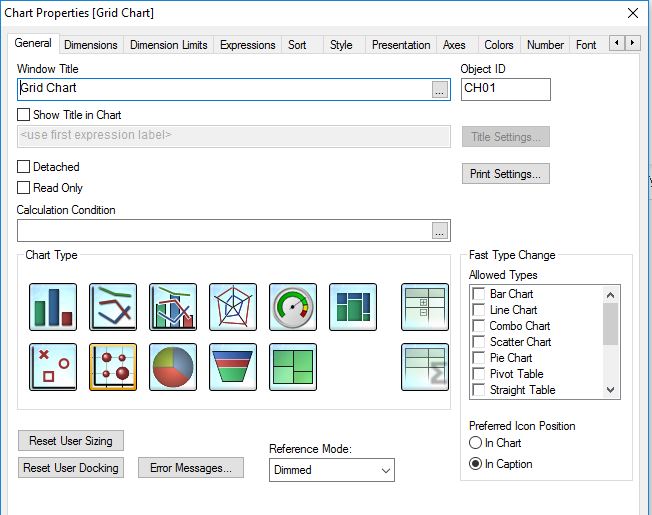
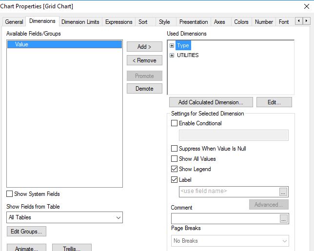
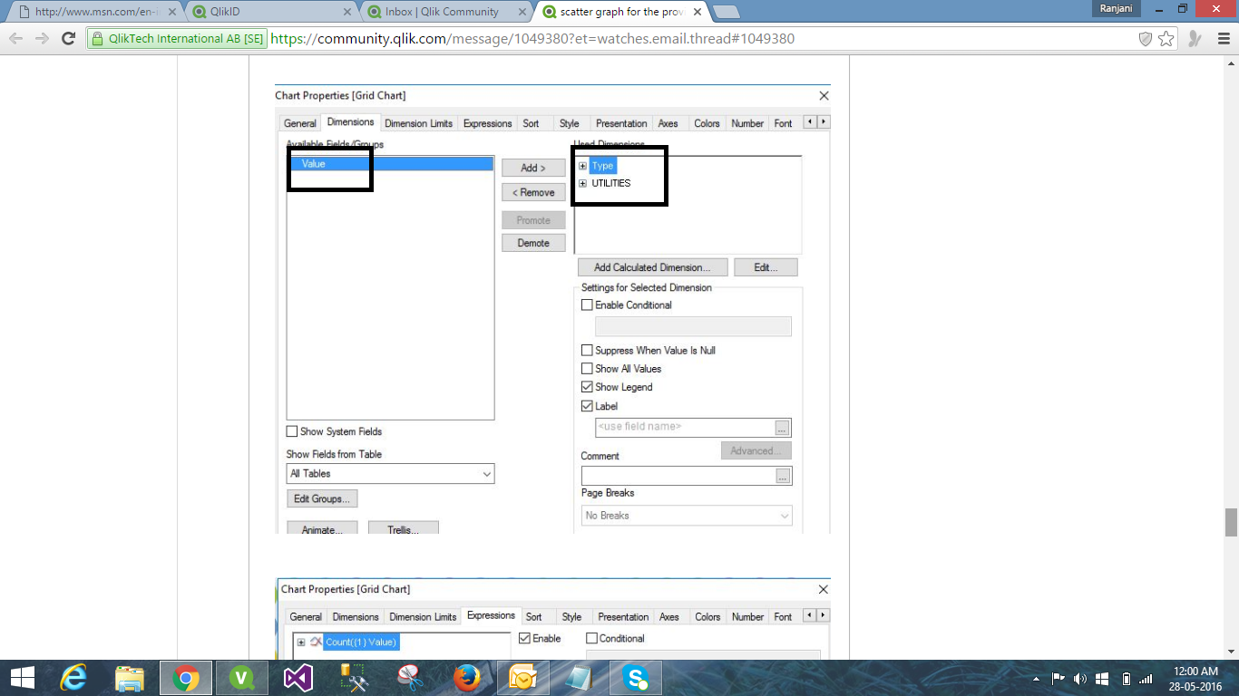
b) Create grid chart with dimensions Type and UTILITIES
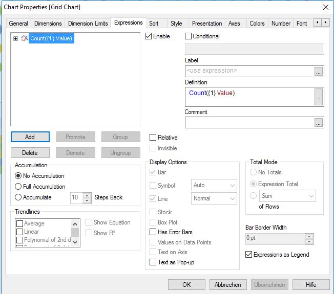
Expression:
=Count({1} Value)
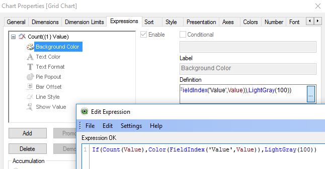
Background color attribute expression:
=If(Count(Value),Color(FieldIndex('Value',Value)),LightGray(100))
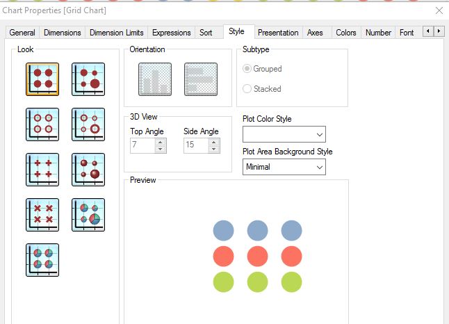
Set the style to the one on the upper left corner.
I think that's mostly it.
For the legend,copy the grid chart and replace the Type dimensions with a calculated
=''
and the UTILITIES dimension with Value
- Mark as New
- Bookmark
- Subscribe
- Mute
- Subscribe to RSS Feed
- Permalink
- Report Inappropriate Content
Hi,
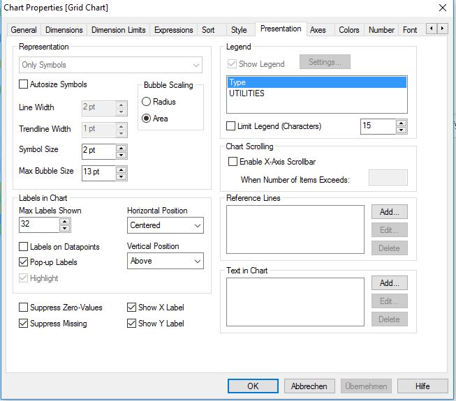
here are some screenshots of the chart properties tabs:
please evaluate the pivot table solution Stefan suggested as well because it can deliver the same colour results including the actual values in each cell.
hope this helps
regards
Marco
- Mark as New
- Bookmark
- Subscribe
- Mute
- Subscribe to RSS Feed
- Permalink
- Report Inappropriate Content
Hi Marco,
thanks a lots for your great support. but one thing i dint understand that Value and type. i have marked it in a black box.
Regards
Ranjani.H.Gowda
- Mark as New
- Bookmark
- Subscribe
- Mute
- Subscribe to RSS Feed
- Permalink
- Report Inappropriate Content
hey swuehl @marco
Thanks a lot to all.for such a great support. This is tremendous team. never seen such a great support to the beginners. Thanks a lot once again.
Regards
Ranjani.H.Gowda
- Mark as New
- Bookmark
- Subscribe
- Mute
- Subscribe to RSS Feed
- Permalink
- Report Inappropriate Content
This screenshots just says that Type and UTILITIES are the two dimensions used in this chart.
What is your question?
regards
Marco
- Mark as New
- Bookmark
- Subscribe
- Mute
- Subscribe to RSS Feed
- Permalink
- Report Inappropriate Content
Value and Type are the two fields created by the CROSSTABLE LOAD prefix.
Have a look at the script(s) I've posted in my first and last post.
- « Previous Replies
- Next Replies »