Rolling average

[hansdevr]

Hi and good morning everyone!

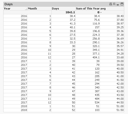
I have a table which shows average project throughput time in days per end of month.

What I would want, is to calculate a "rolling average", but with a twist..

Month 1 should show 38.4, month 2 should show the average of sum of months 1 and 2, and so on.

In the new year, this should be reset and start over again with just the average of month 1.

What would be the best way of achieving this? Through set analysis? Load script?

Any help would be greatly appreciated!

[hansdevr]

Again, this renders the same numbers as found in the column [Throughput time in days]...

[hansdevr]

You were closer the first time.. Now I get "gaps" in the output...

[Frank_Hartmann]

would you be able to share a sample qvw?

[Anil_Babu_Samineni]

Because, you added second issue over initial thread. Can you tell us expected result.

[hansdevr]

You're mistaken. I added nothing.

Month 1 should show 38.4, month 2 should show the average of sum of months 1 and 2, and so on.

In the new year, this should be reset and start over again with just the average of month 1.

This second clause was already there...

[Anil_Babu_Samineni]

That is where it works.. Will you attach excel file instead image so then we can look

[qliksus]

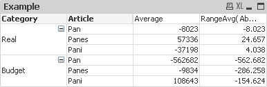
Are you using a straight or Pivot table? If you use  pivot table the rows should be resetted when there is a new value.  Look the  below case when the category field changes it just reset to the new value

RangeAvg( Above(avg({<Y= {$(=Max(Y))}>}amount )-Sum ({<Y= {$(=Max(Y)-1)}>}[Venta Neta]),0,RowNo()))

[mdmukramali]

Dear,

can you try

For Average:

=numavg(above([Throughput time in Days],0,(aggr(RowNo(),Year,Month))))

For Sum:

=numsum(above([Throughput time in Days],0,(aggr(RowNo(),Year,Month))))

Kindly find the attached sample Application.

Thanks,

Mukram

[hansdevr]

[hansdevr]

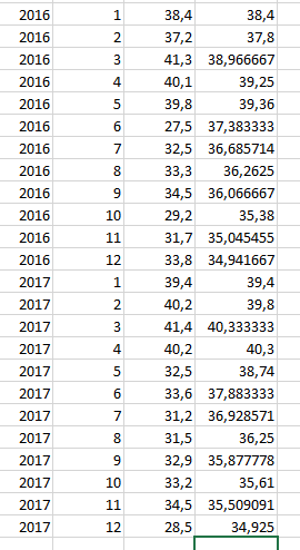
this would be the desired result...