Unlock a world of possibilities! Login now and discover the exclusive benefits awaiting you.
- Qlik Community
- :
- Forums
- :
- Analytics
- :
- New to Qlik Analytics
- :
- Re: Transpose Table
- Subscribe to RSS Feed
- Mark Topic as New
- Mark Topic as Read
- Float this Topic for Current User
- Bookmark
- Subscribe
- Mute
- Printer Friendly Page
- Mark as New
- Bookmark
- Subscribe
- Mute
- Subscribe to RSS Feed
- Permalink
- Report Inappropriate Content
Transpose Table
Hi, I am displaying a table looking like the following:
| Maturity | Sales product1 | Sales product2 | Sales product3 |
| 1 year | 5,913 | 8,133 | -2,223 |
| 2 year | 39,525 | 38,560 | 929 |
| 3 year | 41,094 | 39,872 | 1,188 |
| 4 year | 97,904 | 79,516 | 4,737 |
| 5 year | 309,085 | 290,612 | 9,810 |
| 6 year | 85,371 | 109,481 | 2,710 |
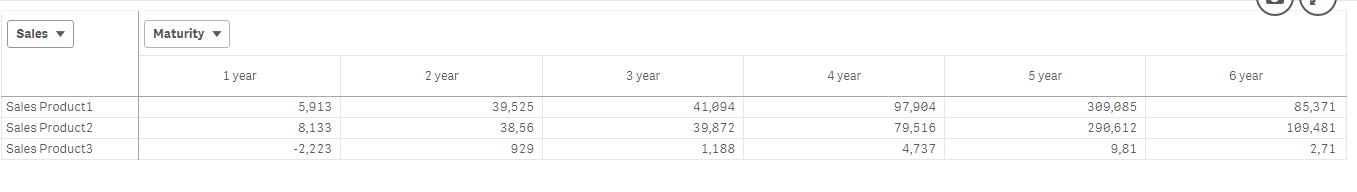
That I would like to transpose to look like this:
| Maturity | 1 year | 2 year | 3 year | 4 year | 5 year | 6 year |
| Sales product1 | 5,913 | 39,525 | 41,094 | 97,904 | 309,085 | 85,371 |
| Sales product2 | 8,133 | 38,560 | 39,872 | 79,516 | 290,612 | 109,481 |
| Sales product3 | -2,223 | 929 | 1,188 | 4,737 | 9,810 | 2,710 |
Any suggestions to do this please. Thanks very much.
- « Previous Replies
-
- 1
- 2
- Next Replies »
- Mark as New
- Bookmark
- Subscribe
- Mute
- Subscribe to RSS Feed
- Permalink
- Report Inappropriate Content
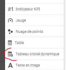
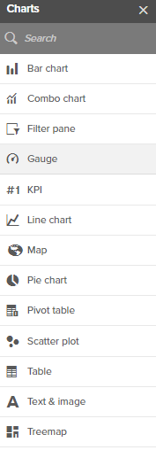
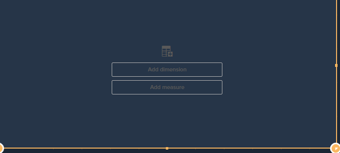
Create a pivot table:
as a dimension:
=ValueList('Sales Product1','Sales Product2','Sales Product3')
as a measure:
if(ValueList('Sales Product1','Sales Product2','Sales Product3')='Sales Product1', sum([Sales product1]),
if(ValueList('Sales Product1','Sales Product2','Sales Product3')='Sales Product2', sum([Sales product2]),
if(ValueList('Sales Product1','Sales Product2','Sales Product3')='Sales Product3', sum([Sales product3]))))
add a line:
Maturity
RESULT:
- Mark as New
- Bookmark
- Subscribe
- Mute
- Subscribe to RSS Feed
- Permalink
- Report Inappropriate Content
Thanks very much Omar. if i understood correctly, i go to charts, and select Pivot table
open it and fill it using the code you suggested by adding a dimension
- Mark as New
- Bookmark
- Subscribe
- Mute
- Subscribe to RSS Feed
- Permalink
- Report Inappropriate Content
Yes please
- Mark as New
- Bookmark
- Subscribe
- Mute
- Subscribe to RSS Feed
- Permalink
- Report Inappropriate Content
Script / Front end?
- Mark as New
- Bookmark
- Subscribe
- Mute
- Subscribe to RSS Feed
- Permalink
- Report Inappropriate Content
Hi,
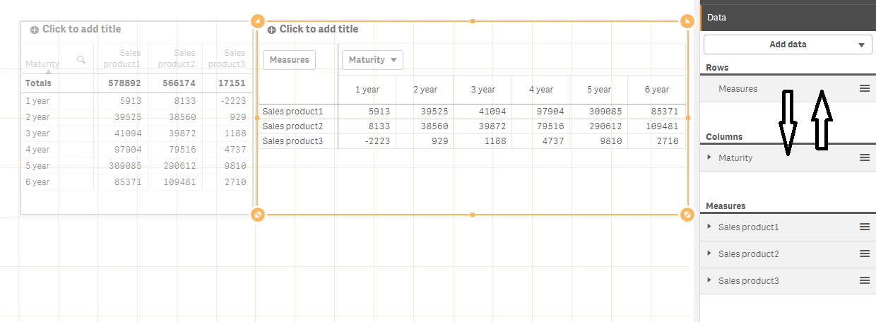
You can achieve that by just converting your table to pivot table and switch column and rows. That's all you need
- Mark as New
- Bookmark
- Subscribe
- Mute
- Subscribe to RSS Feed
- Permalink
- Report Inappropriate Content
Never thought this was possible ! Thanks a lot !
- Mark as New
- Bookmark
- Subscribe
- Mute
- Subscribe to RSS Feed
- Permalink
- Report Inappropriate Content
Hi,
As Kaan rightly suggested, you can do it by simply creating a pivot chart and transposing your measures and Dimension.
But an alternate way to do this is in the script as well. PFA images for your reference.
Scripting :-

Output:-

Regards,
Saniya.
- Mark as New
- Bookmark
- Subscribe
- Mute
- Subscribe to RSS Feed
- Permalink
- Report Inappropriate Content
Thanks Kaan. Can you please explain how to convert an existing table to pivot table ?
I have tried to create a new pivot table and flipped the columns into rows but did not get the right results. the reason being that the Sales Product columns don’t exist already in the tables, but I create them on the fly using formulas like
=sum(if([Product]='Product1', [Sales])) for Sales product1 column.
=sum(if([Product]='Product2', [Sales])) for Sales product2 column
=sum(if([Product]='Product3', [Sales])) for Sales product3 column
- Mark as New
- Bookmark
- Subscribe
- Mute
- Subscribe to RSS Feed
- Permalink
- Report Inappropriate Content
Hi,
You can just drag a Pivot Table over a Table as select Convert if you want to convert it but you may have to review the default design and may not get exactly what you want right away.
To create from scratch just try something simpler:
Dimension: Product
Measure: Sales and select Sum
Then Add Data (Column) and select Year
Then, if you want, you can restrict Sales to specific products by editing the Measure and changing it from
Sum(Sales)
to
Sum({<Product={"Product1","Product2","Product3"}>} Sales)
I hope this helps,
Luis
- « Previous Replies
-
- 1
- 2
- Next Replies »