Color a Pivot Table

[antoniodneto]

Hello Guys.

I need your help.

I have one pivot table where DATA_BASE is my Dimension, and some rows.

Each row has your specific expression to calc.

I'm trying to find a way to color the values in the row, where highers in red,medium yellow and lowers in green. Making a gradient among them.

My app is attached to understand my view.

Thank you so much guys!!!

[jonvitale]

Okay, so here's what it looks like:

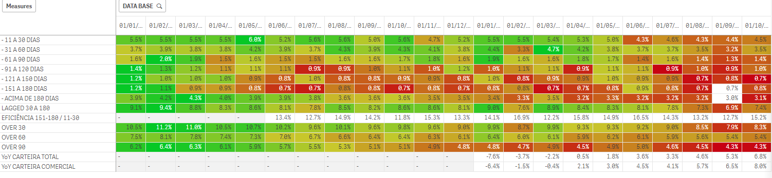
I updated the variables to reflect the new measures without the "before" function. I couldn't do so with rows 9, 13, or 14, so they don't have a color.

Here's what the formula looks like in each:

If ( ($(vM1) - Min(total Aggr($(vM1), DATA_BASE))) / (Max(total Aggr($(vM1), DATA_BASE)) - Min(total Aggr($(vM1), DATA_BASE))) < 0.5, 
ColorMix1(
($(vM1) - Min(total Aggr($(vM1), DATA_BASE))) / (Max(total Aggr($(vM1), DATA_BASE)) - Min(total Aggr($(vM1), DATA_BASE))) * 2
        , $(vColor_Low), $(vColor_Mid)
    ),
    ColorMix1(
(($(vM1) - Min(total Aggr($(vM1), DATA_BASE))) / (Max(total Aggr($(vM1), DATA_BASE)) - Min(total Aggr($(vM1), DATA_BASE))) - 0.5) * 2
        , $(vColor_Mid), $(vColor_High)
    )
)

The interesting part here is the Aggr expressions. Basically, what I am doing is asking Qlik to apply my measure $(vM1) to each value of the DATA_BASE dimension. Then I take either the Min or the Max of these values. I need the keyword "total" in the Min or Max function to ensure that the AGGR function will work on all values of DATA_BASE and not just the one we are in at this cell value.

Let me know if you have any questions about how this works. Hopefully, this will solve the problem.

[jonvitale]

Ah, that's good stuff. Wish you'd seen this four days ago.

[antoniodneto]

Kaan,

Great!!! Is exactly what I am looking for.

One question?

I couldn't apply in the rows "EFICIENCIA 151-180/11-30" "YoY CARTEIRA TOTAL" and "YoY CARTEIRA COMERCIAL"

Can you help me to solve them?

[antoniodneto]

Hey Kaan!! I GOT!!!!

Thank you so much!!

Jonathan,

Thank you so much for you time, work and patience. Sorry for anything.

You guys are great!!!

[colinodonnel]

That formula is brilliant.

ColorMix2( (hrank(total {{Measure Expression}} )/(NoOfColumns(TOTAL)/2))-1 ,red(), green(),Yellow())

To apply it  per column (min/max each column), simply replace NoOfColumns with NoOfRows