Urgent: Pivot Chart Above and Below Average

[#1]

Hi all,

I need your help. I have a pivot chart which has two dimensions (Region and Branch) and i have two measures V1 and V2. I want to create another pivot chart with only Region and three variables Count of distinct branches, V2 above 10 and V2 below 10. The description of the pivot charts and the desired final pivot charts are presented in the attached excel. I am new to Qlikview, Can you please share an example of how i can create this view?

Thanks a lot for your help!

- Harsha

[swuehl]

Try creating a chart with dimension Region and three expressions:

=count(distinct Branch)

=count({<V2 = {">=10"}>} distinct Branch)

=count({<V2 = {"<10"}>} distinct Branch)

Hope this helps,

Stefan

edit:

You probably want a larger than / equal for the above10 expression

[#3]

The way that Stefan Said is the correct butI think you also need to change your field Region in your excel, like the one I attached.

Greetings!!

[#4]

Thank you Javierortiz and Stefan for your responses.

The solution you have provided works perfectly when V2 is a part of the input data. In my case the field V2 is not a part of my data, i am creating this field using several formula in the pivot chart.

I am not sure as to how i can use an expression already defined in a set analysis expression. For example when i try and create one more field, a new variable V3 which is sum(V2) and use it as "=Count({<[V3]={">=10"}>}DISTINCT Branch)" both the counts are showing the same value.

I really appreciate your help in this regard.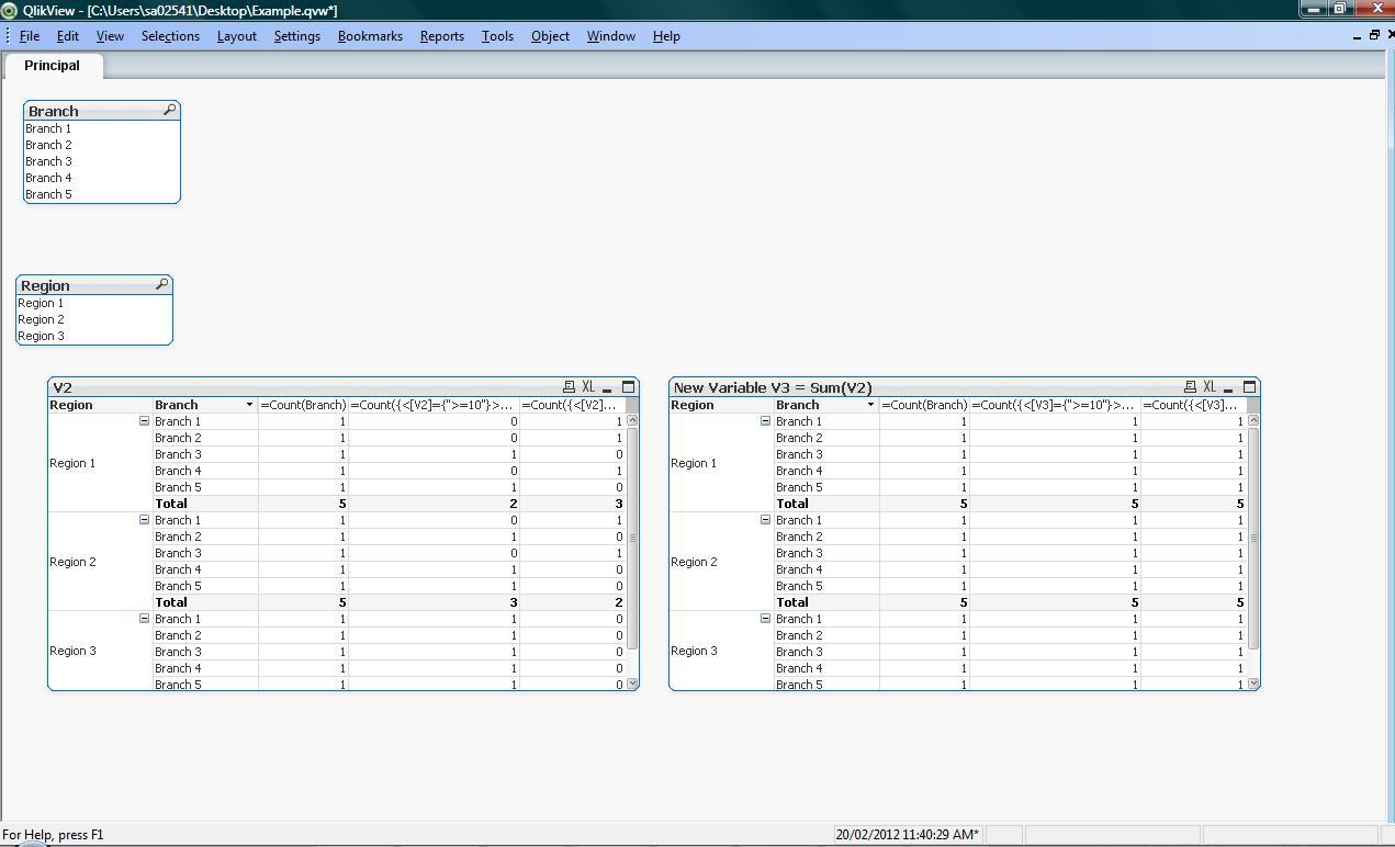

Thank you! 

- Harsha

[swuehl]

I assume that the set expression is completely ignored because of some problem with your [V3] field. Where and how have you declared the field [V3]? In the script? How does your load look like?

It would be useful to know how your definition of V2 looks like, too. Could you maybe upload a small sample file?

Regards,

Stefan

[#6]

you meant something like this?

[#7]

Hi,

Let me try and explain my scenario. The attached image shows three tables:

Existing Pivot Chart: I have created this pivot chart. In this chart V1 is a field that i have created using the raw data. # Branches >10 takes the value 1 when V1 >10, similarly #Branches < 10 takes the value 1 when V1<10.

Desired Reporting Level with wrong numbers: I want to report the numbers at a region level, where i want to count the number of branches and and within them i want to show how many are ">10" and "<10". But when i remove the Branch dimension from the pivot chart the value of V1 becomes 53.3 and so both my values "# Branches >10" and "#Branches < 10" become 13 and 0 respectively which is not what i want.

Desired Reporting Level with correct numbers: What i wanted to finally have is shown in this table where i want to report the numbers at a region level but want to show the number of branches which are above and below: 6 and 7 respectively.

I am not sure as to how this can be done using qlikview. I hope i am clear. I really appreciate any help in this regard. Iam new to qlikview,it would be great if you can post an example showing how i can accomplish this.

Thank you!

- Harsha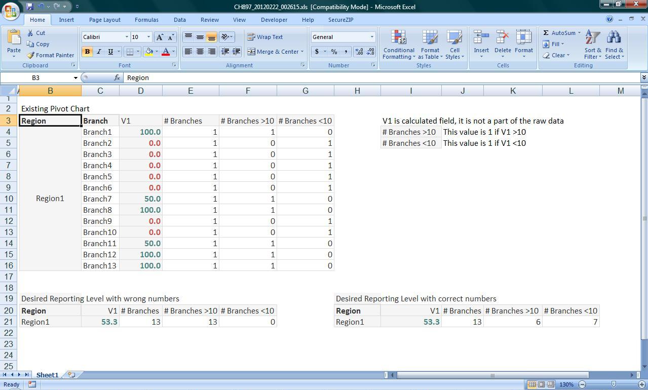

P.S. I wanted to attach the excel but i could not find a provision for document attachment here. So i have attached the image.

[swuehl]

Hi,

the file upload is available in advanced editor, link at upper right in editor (or if you modify an existing post).

Try something like

=sum( aggr( count(distinct if(V1 >=10, Branch)), Region, Branch))

as expression in your new table.

V1 is just a field value, no aggregation needed per Branch, right?

Hope this helps,

Stefan