Unlock a world of possibilities! Login now and discover the exclusive benefits awaiting you.
- Qlik Community
- :
- All Forums
- :
- QlikView App Dev
- :
- Creating a trailing 52 week chart
- Subscribe to RSS Feed
- Mark Topic as New
- Mark Topic as Read
- Float this Topic for Current User
- Bookmark
- Subscribe
- Mute
- Printer Friendly Page
- Mark as New
- Bookmark
- Subscribe
- Mute
- Subscribe to RSS Feed
- Permalink
- Report Inappropriate Content
Creating a trailing 52 week chart
Hi
I'm trying to create a chart which shows the trailing 52 week total for a variable (in this example Sales). Basically, on the chart below, the value for weekname 2004/01 is the sum of that week's sales plus the previous 51 weeks' sales, for 2013/52 it is the sum of that week and the previous 51 weeks sales. I also want to restrict the view to the last 26 weeknames. The attached spreadsheet gives an example of the data and the graph I'm trying to create.
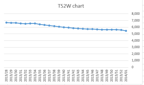
I have tried using the formula: Rangesum(Above(Total sum(Sales),0,52)) which works fine until I apply the dimension limit of using the first 26 values! I've mucked around with various options, but have now hit a brick wall.
All ideas & help greatly appreciated!
thanks
Richard
Accepted Solutions
- Mark as New
- Bookmark
- Subscribe
- Mute
- Subscribe to RSS Feed
- Permalink
- Report Inappropriate Content
In QV, we can set it to display a scroll bar, but default it to display the last 26 values:
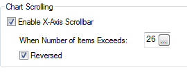
This will accumulate it correctly, while still only showing the last 26 values on default (giving the user the ability to go back further in time if they so wish). See the attached for full example.
If you don't want to go this route, I believe you will need to calculate the rolling average in your load script instead of in the chart itself.
- Mark as New
- Bookmark
- Subscribe
- Mute
- Subscribe to RSS Feed
- Permalink
- Report Inappropriate Content
In QV, we can set it to display a scroll bar, but default it to display the last 26 values:
This will accumulate it correctly, while still only showing the last 26 values on default (giving the user the ability to go back further in time if they so wish). See the attached for full example.
If you don't want to go this route, I believe you will need to calculate the rolling average in your load script instead of in the chart itself.
- Mark as New
- Bookmark
- Subscribe
- Mute
- Subscribe to RSS Feed
- Permalink
- Report Inappropriate Content
Thanks Nicole.
Sorted!