Conditional Formatting of a Dimension in a Pivot Table

[justin_morley]

Hi,

I need to conditionally format a dimension in a Privot Table, could somebody point me in the right direction?

My data looks very approximately like this:

dimension	flag	expression
1	0	87
2	1	56
3	0	12.1

I require conditional formatting to be placed on the dimension so that 1 and 3 are black and 2 is light grey, because of the value in the flag.

What I've tried so far:

1) Chart Properties>Dimensions>Used Dimensions -> expand the dimension and create the following expression under Text Color

=if(flag=1,LightGray(),Black())

This is completely ignored, as is =LightGray() or just Gray()

Why is this option even there if it doesn't work? Is there a switch somewhere I'm missing

2) Turn On Design Grid>Right Click in Cell>Select Custom Format Cell>Select Text Color>Base Color>Calculated and insert the same expression:

=if(flag=1,LightGray(),Black())

This time LightGray() on its own works, but the conditional expression does not.

Anyone know how I can acheive the conditional formatting I need? Looking through the archives I haven't found a satisfactory answer.

I'm on 11.20 SR5

Thanks,

Justin

[justin_morley]

I've got it!

The answer is it only applies the formatting if there is something in the first pivoted field. there is a great deal of white space in my pivot table (which is desirable and unavoidable ) and it looks more like this:

dimension	flag	pivot dimension	pivot value 1	pivot value 2
1	0
2	1			12.3
3	0
4	0
5	0		87	8
6	0		56

The first pivot value only has data against dimensions 5 and 6, and thus the formatting is only applied to dimensions 5 and 6.

However, I've failed to recreate these conditions in a stand alone app, so there must be something else going on here. Does this new information jog anybody's mind?

[kuba_michalik]

Dammit, and here I was just about to post the solution

However, a part of it still might be useful to you. I have no idea if it is really true, but it appears as if the conditional formatting expressions for dimensions are evaluated as if they were put on the first column of the chart. If that first column would happen to contain a missing combination of dimensions, tough luck Even an unconditional expression would get ignored in such case.

Hovewer, in this context, this:

flag=1

is for practical purposes shorthand for this:

Only(flag)=1

and that fact gives us a bit more control.

I assume you want to consider value of flag as in relation to the value of dimension only, so this:

If(Only(TOTAL<dimension> flag)=1,LightGray(),Black())

could be just what you are looking for.

Edit: it also needs to have "Populate missing cells" to work. If first expression column contains actual missing values, nothing can help. I attached a small example.

Edit2: It seems I overcomplicated this. Looks like "Populate missing cells" is all that is needed.

[justin_morley]

Great stuff! Thanks so much for this analysis and test app. Getting there by degrees!

Setting "Populate Missing" allows an unconditional expression on a dimension to work for me

However the conditional bit still fails to evaluate for some reason. Any ideas? I now have a reduced app which exhibits this behaviour but I'm reluctant to attach it due to data sensitivity. I may have a go at obfuscating the data and posting the app.

Thanks for your help,

Justin

[kuba_michalik · Accepted solution]

If flag is associated with [dimension], but not necessarily with every combination of [dimension] and other pivot dimensions, then 'flag' in conditional expression could still evaluate to null and cause the test to fail - expression technically works,but you get the 0-flag color anyway. This is a part where the Only(TOTAL<dimension> flag) bit actually comes helpful. I'm attaching an example, hope it helps.

[justin_morley]

Bingo! You are a very clever man my friend!

The combination of "Populate missing cells" and your Only(TOTAL<dimension> flag) wizardry works a treat.

Now to spend a few hours trying to get my head around exactly what that expression is doing...

Thanks so much for your help.

[anilet123]

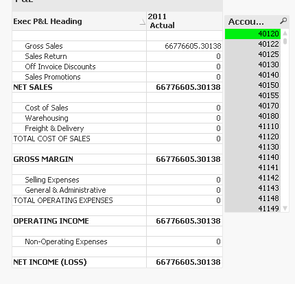
Hi Jakub,

I tried the following expression in my PL Statement(straight table), it did not work for me when made selections on filters.

if(Only(TOTAL<[Exec P&L Heading]>[Exec P&L Calculation])='c' ,'<B>')

I had selected Account Number, the format bold disappeared for "TOTAL COST OF SALES " and " TOTAL OPERATING EXPENSES". Irrespective of the selections I would want the format to be unchanged.

Could you please help on this?

Regards,

Anilet Nirmal

[anilet123]

Hi,

I got the solution. I applied the condition if(Only({<[Account Number]=>}[Exec P&L Calculation])='c' ,'<B>')  and it works fine.

Thanks.

Regards,

Anilet Nirmal