Pivot table with set analysis

[#1]

Hi everybody! I have some problem with such task:

we have a table with data:

Header 1	Header 2	Header 3	Header 4
ClientID	ReceiptSum	ReceiptInterval	Date
11	101	100-200	01/01/2014
11	120	100-200	01/02/2014
11	50	0-100	02/02/2014
22	70	0-100	01/05/2014
22	150	100-200	10/01/2014

so the task is to build a pivot table like that:

Header 1	Header 2	Header 3	Header 4
ReceiptInterval	100-200	1	1
	0-100	2 (number of customers)	0
		1	2
		count of receipts

I tried several ways to build that table:

1)-in data model create table

Load

Count (ClientID) as Count_of_receipts,

ClientID ,

ReceiptInterval

resident TotalReceipts Group by ReceiptInterval, ClientID;

then use this table for building pivot tavle. It works but pivot table is insensitive to selections made by user.

2)- make table of several text objects, in each object i'll calculate certain value, for eaxmple: calculate number of customers, who have 1 receipt in the amount of 100-200, than calculate number of customers,who have 2 receipts in the amount of 100-200 etc. For such calculations I I've used set analysis, but it doesn't work.

=Count({$<ReceiptInterval={'100-200'}, count({<ReceiptInterval={'100-200)>}ReceiptInterval={1})>}distinct ClientID )

Can anybody help with this expression or another way to solve my problem? Thanks in advance!

[MK_QSL]

Sorry but I am still unclear due to your format of excel file.

If you give us exact format then only can help you.

[#3]

[#4]

am also confused please have look at images

[#5]

Exact format is in Example.xlsx. this is how table should look like. in Example.qvw is my variant of this table, but it doesn't suit, because of insensitivity to current selection. Can you clearify what exactly is unclear?

[#6]

Ok, lets try to explain how I tried to solve the problem.

Table with data

Header 1	Header 2	Header 3	Header 4
ClientID	ReceiptSum	ReceiptInterval	Date
11	101	100-200	01/01/2014
11	120	100-200	01/02/2014
11	50	0-100	02/02/2014
22	70	0-100	01/05/2014
22	150	100-200	10/01/2014

I transformed to another table in script reload

Load

Count (ClientID) as Count_of_receipts,

ClientID ,

ReceiptInterval

resident TotalReceipts Group by ReceiptInterval, ClientID;

Result is next:

Calc_Table:

Header 1	Header 2	Header 3
Count_of_receipts	ClientID	ReceiptInterval
1	11	0-100
2	11	100-200
1	22	0-100
1	22	100-200

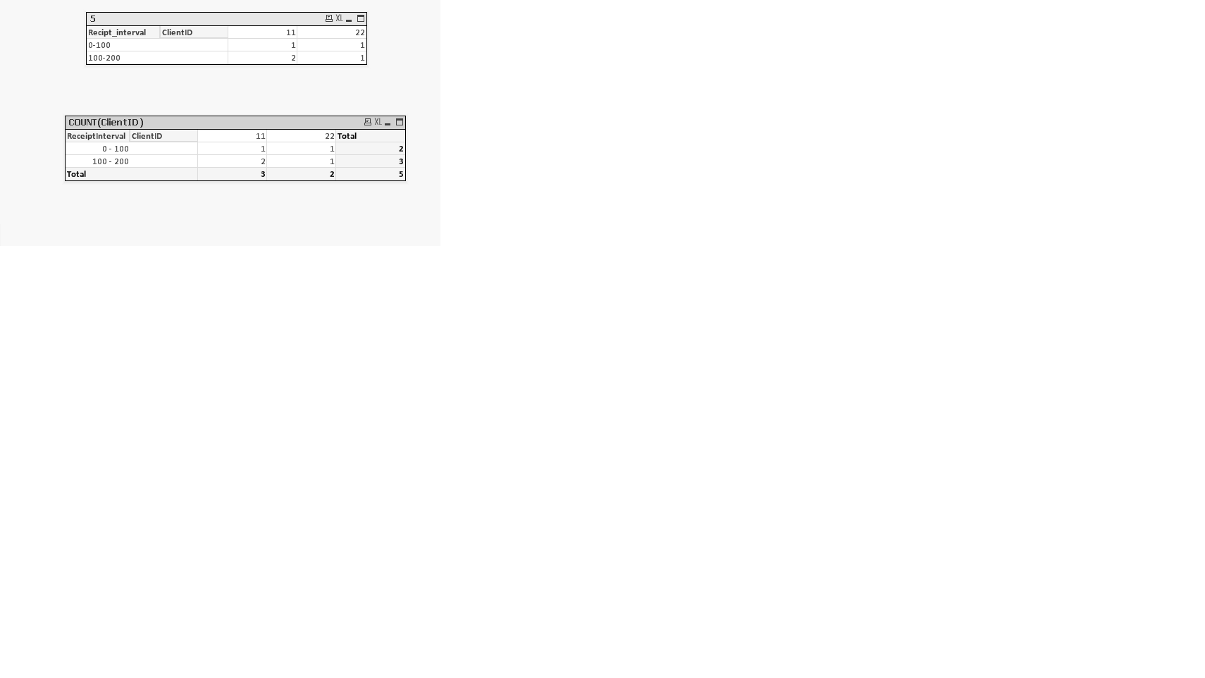
Then using this Calc_Table i build the pivot table

dimensions:

-count_of_receipts

-ReceiptInterval

expression: count(ClientID). as it should look like (see images and examples)

BUT. Because of calculation table in script I can't update pivot table after selections

[#7]

So, finally I built required table, but in very unusual way. Basically it is not a table,but 2dimension array of text objects. Every object contains expression like:

=Count ({$}If(Aggr(Count({$<ReceiptInterval={'100-200'}>}card_number),card_number)=1,card_number) )

Next object has the same expression, but with another ReceiptInterval and\or Count value:

=Count ({$}If(Aggr(Count({$<ReceiptInterval={'200-300'}>}card_number),card_number)=1,card_number) )

=Count ({$}If(Aggr(Count({$<ReceiptInterval={'200-300'}>}card_number),card_number)=2card_number) )

=Count ({$}If(Aggr(Count({$<ReceiptInterval={'200-300'}>}card_number),card_number)=3card_number) )

This "table" doesn't work very fast, but it is the only way i found...