Unlock a world of possibilities! Login now and discover the exclusive benefits awaiting you.
- Qlik Community
- :
- All Forums
- :
- QlikView App Dev
- :
- Re: Area Chart(or line chart) in chart table
Options
- Subscribe to RSS Feed
- Mark Topic as New
- Mark Topic as Read
- Float this Topic for Current User
- Bookmark
- Subscribe
- Mute
- Printer Friendly Page
Turn on suggestions
Auto-suggest helps you quickly narrow down your search results by suggesting possible matches as you type.
Showing results for
Not applicable
2014-04-11
01:40 AM
- Mark as New
- Bookmark
- Subscribe
- Mute
- Subscribe to RSS Feed
- Permalink
- Report Inappropriate Content
Area Chart(or line chart) in chart table
Hi All
Now I have a serious steps in Excel:
1. Original Table
| Year | Product | Grade |
| 2011 | 1 | A |
| 2011 | 2 | A |
| 2011 | 3 | B |
| 2011 | 4 | B |
| 2011 | 5 | B |
| 2011 | 6 | C |
| 2011 | 7 | C |
| 2011 | 8 | C |
| 2011 | 9 | C |
| 2010 | 10 | A |
| 2010 | 11 | B |
| 2010 | 12 | B |
| 2010 | 13 | C |
| 2010 | 14 | C |
| 2010 | 15 | C |
| 2009 | 16 | A |
| 2009 | 17 | A |
| 2009 | 18 | A |
| 2009 | 19 | A |
| 2009 | 20 | B |
| 2009 | 21 | C |
2.
| 2011 | 2010 | 2009 | |
| A | 2 | 1 | 4 |
| B | 3 | 2 | 1 |
| C | 4 | 3 | 1 |
| Total | 9 | 6 | 6 |
3.
| 2011 | 2010 | 2009 | |
| A | 22% | 17% | 67% |
| B | 33% | 33% | 17% |
| C | 44% | 50% | 17% |
| Total | 100% | 100% | 100% |
4.And Then I could insert a line chart:

And My question is How can I just load the original data from my data source and insert the final area chart directly?
660 Views
- « Previous Replies
-
- 1
- 2
- Next Replies »
10 Replies
Not applicable
2014-04-11
02:27 AM
Author
- Mark as New
- Bookmark
- Subscribe
- Mute
- Subscribe to RSS Feed
- Permalink
- Report Inappropriate Content
I have tried but i doesn't work. I would like the final chart like this .....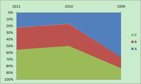
38 Views
- « Previous Replies
-
- 1
- 2
- Next Replies »