Unlock a world of possibilities! Login now and discover the exclusive benefits awaiting you.
- Qlik Community
- :
- All Forums
- :
- QlikView App Dev
- :
- Re: different row colors pivot table
- Subscribe to RSS Feed
- Mark Topic as New
- Mark Topic as Read
- Float this Topic for Current User
- Bookmark
- Subscribe
- Mute
- Printer Friendly Page
- Mark as New
- Bookmark
- Subscribe
- Mute
- Subscribe to RSS Feed
- Permalink
- Report Inappropriate Content
different row colors pivot table
Can I in a pivot table make that the rows have different colors.
Like:
row 1 : dark blue
row 2: light blue
row 3: dark blue
row 4: light blue
etc.
- Mark as New
- Bookmark
- Subscribe
- Mute
- Subscribe to RSS Feed
- Permalink
- Report Inappropriate Content
Enter in the 'Background Color' expression for your dimensions/expression and use something like:
If(Mod(RowNo(), 2) > 0, LightBlue(), Blue())
- Mark as New
- Bookmark
- Subscribe
- Mute
- Subscribe to RSS Feed
- Permalink
- Report Inappropriate Content
Hi,
you could also use (change Gray to Blue:
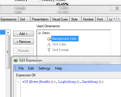
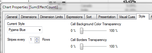
against each dimension and expression in your chart. OR you can just set 'Current Style' on the Style tab to be 'Pyjama Blue'
HTH
Andy
- Mark as New
- Bookmark
- Subscribe
- Mute
- Subscribe to RSS Feed
- Permalink
- Report Inappropriate Content
Than become all the cells with a number darkgrey and the ones with no number stay white.
- Mark as New
- Bookmark
- Subscribe
- Mute
- Subscribe to RSS Feed
- Permalink
- Report Inappropriate Content
It won't colour a cell if it's a null - also, I don't think you can use the 'stripes every'...for pivot tables.
You can try 'populate missing cells' and enter a value to force it to colour those cells, or depending on what you're loading and pivoting, consider using a null as value tin your script o give a value to those that are missing.
- Mark as New
- Bookmark
- Subscribe
- Mute
- Subscribe to RSS Feed
- Permalink
- Report Inappropriate Content
'against each dimension and expression in your chart. OR you can just set 'Current Style' on the Style tab to be 'Pyjama Blue'' This is impossible by pivot tables.
- Mark as New
- Bookmark
- Subscribe
- Mute
- Subscribe to RSS Feed
- Permalink
- Report Inappropriate Content
PFA
- Mark as New
- Bookmark
- Subscribe
- Mute
- Subscribe to RSS Feed
- Permalink
- Report Inappropriate Content
Hi,
Option 1 - In Style tab, Select current style - Pyjama Blue option with Strip 1 , 2.
If it doesn't solve your purpose then use Option 2
Option 2 - Use custom conditions on background color (both dimensions and expression to highlight entire row)
For eg. =if(Match( [Column Name], 'Field1','Field1','Field1') , RGB(102,102,255)) or if else statement.
Regards,
Kuldeep
- Mark as New
- Bookmark
- Subscribe
- Mute
- Subscribe to RSS Feed
- Permalink
- Report Inappropriate Content
First option is IMPOSSIBLE by pivot tables I think!
Second options do not work!