Show all values in Pivot table when field selected

[nsm1234567]

Hi There,

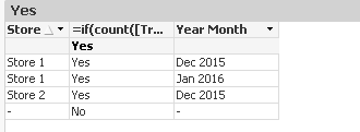
I'm hoping someone can assist with an issue I'm having.  In the attached QVW I have a pivot table with an expression that looks as follows:  =if(count([Transaction Date])>0,'Yes','No')

When looking at all the stores, this works fine, however, if I select "Store 2" only the Dec 2015 value is shown in the pivot table, as "Jan 2016" isnt a possible month when this store is selected.  Is there any way around this?  In other words, is there a way for me to show both Jan 2015 and Dec 2015 when store 2 is selected (where the value in Jan 2015 would be "No")?  Any help would be greatly appreciated.

Below is the load script from my example:

TransactionTable:

LOAD * INLINE [

    Transaction Date, Store

    2015/12/17, Store 1

    2015/12/18, Store 2

    2016/01/16, Store 1

];

DatesTable:

LOAD * INLINE [

    Transaction Date, Year Month

    2015/12/17, Dec 2015

    2015/12/18, Dec 2015

    2016/01/16, Jan 2016

];

[Anonymous]

Show all values in Pivot/Straight Table (irrespective of current selection)

I think this link will get you what you need.  I used this method to solve a problem a while back

[#3]

if you make your chart a stright table and select show all values for the dimension it looks like the date is not showing for the No

[#4]

since QV is building based on what is associated with the dates and there is nothing for store 2 in Jan 2016 -

I would suggest building a mini calendar and count that way

The data model needs to be updated so it would have 4 rows in a stright table or table box for example showing the count for each store in each year

[nsm1234567]

Hi There,

Thanks for the reply.  Would you be able to illustrate how this would work in the attached app?  I've tried a few scenarios but they didn't work

[nsm1234567]

Hi There,

As mentioned, I realise that the reason Jan 2016 is shown is because it is not a possible "Year Month" when the selection is made.  However, Qlikview is evaluating the result when nothing is selected, and I'd like it to be "forced" to evaluate regardless of whether the store is selected or not.  Unfortunately, the actual dataset is a lot more complex than what I've presented here, which is why I'm trying to accomplish this on the front-end.

[Anonymous]

Yes.  I can do that, but I won't be able to review your qvw until tomorrow.  However, the crux of what you need to understand is this.  The formula needs to compare your selected total to the overall document total ignoring your dimension and then be able to assign a zero (0) as a value rather than a null.  Nulls get ignored in a pivot table, but zeros can get displayed, thus showing all of your dimensions rather than only those with data

Here is an example of a formula that I use to solve a similar problem.

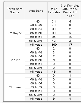
if(count({1}[Member Counter]) <> count([Member Counter]),count({<[CDM Lives]={'CDM Lives'}>}[Member Counter]),0)

You can see in my pivot table example that I have two dimensions, enrollment status and age band.  There are many age bands with zero count of females.  Until I added this formula, it would only display the enrollments and ages that had actual values.   Ignore the set analysis for CDM Lives.

You should be able to use this as a model to solve your problem as it is the same principal

Hope this helps for now and I will check in tomorrow to see if you did not get it.

[Gabriel]

Hi,

Why not try this expression

=if(count({1}[Transaction Date])>0,'Yes','No')

[Anonymous]

This formula seems to solve your problem

=if(count({1}[Year Month]) >0,if(count([Transaction Date])>0,'Yes','No'),'No')

So, if the count of Year Month is greater than zero in all of the data, then it evaluates the next if statement, if not, then it defaults to No which is a value that can be displayed in your table.  I have attached an updated version of your example with the changes.

A pivot table will display all of the values of a dimension as long as there is valid data for each value.  This insures that each dimension value in valid

Hope this gets you what you need