Unlock a world of possibilities! Login now and discover the exclusive benefits awaiting you.
- Qlik Community
- :
- Blogs
- :
- Technical
- :
- Design
- :
- A Myth About Count(distinct …)
- Subscribe to RSS Feed
- Mark as New
- Mark as Read
- Bookmark
- Subscribe
- Printer Friendly Page
- Report Inappropriate Content
Do you belong to the group of people who think that Count(distinct…) in a chart is a slow, single-threaded operation that should be avoided?
If so, I can tell you that you are wrong.
Well - it used to be single-threaded and slow, but that was long ago. It was fixed already for – I think – version 9, but the rumor of its slowness lives on like an urban myth that refuses to die. Today the calculation is multi-threaded and optimized.
To prove that Count(distinct…) is faster than what many people think, I constructed a test which categorically shows that it is not slower – it is in fact a lot faster than the alternative solutions.
I created a data model with a very large fact table: 1M, 3M, 10M, 30M and 100M records. In it, I created a secondary key, with a large number of distinct values: 1%, 0.1% and 0.01% of the number of records in the fact table.
The goal was to count the number of distinct values of the secondary key when making a selection. There are several ways that this can be done:
- Use count distinct in the fact table: Count(distinct [Secondary ID])
- Use count on a second table that just contains the unique IDs: Count([Secondary ID Copy])
- Use sum on a field that just contains ‘1’ in the second table: Sum([Secondary ID Count])
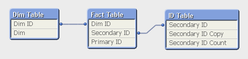
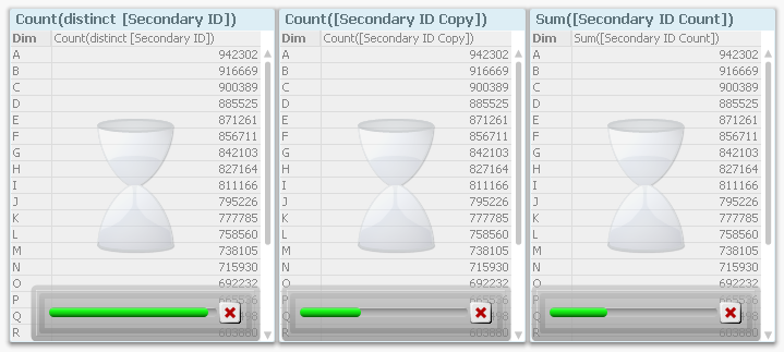
I also created a dimension ("Dim" in the “Dim Table”) with 26 values, also randomly assigned to the data in the fact table. Then I recorded the response times for three charts, each using “Dim” as dimension and one of the three expressions above. I made this for four different selections.
Then I remade all measurements using “Dim ID” as dimension, i.e. I moved also the dimension to the fact table. Finally, I loaded all the recorded data into QlikView and analyzed it.
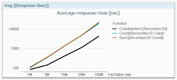
The first obvious result is that the response time increases with the number of records in the fact table. This is hardly surprising…
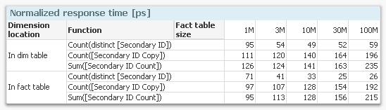
…so I need to compensate for this: I divide the response times with the number of fact table records and get a normalized response time in picoseconds:
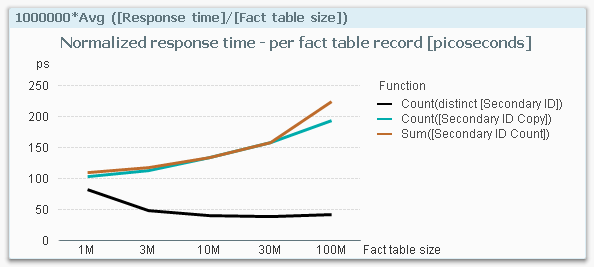
This graph is extremely interesting. It clearly shows that if I use a Count(distinct…) on the fact table, I have a response time that is considerably smaller than if I make a count or a sum in a dimensional table. The table below shows the numbers.
Finally, I calculated the ratios between the response times for having the dimension in the fact table vs. in a dimensional table, and the same ratio for making the aggregation in the fact table vs. in a dimensional table.
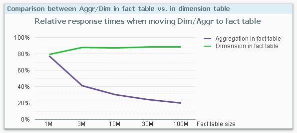
This graph shows the relative response time I get by moving the dimension or the aggregation into the fact table. For instance, at 100M records, the response time from a fact table aggregation (i.e. a Count(distinct…)) is only 20% of an aggregation that is made in a dimensional table.
This is the behavior on my mock-up data on my four-core laptop with 16GB. If you make a similar test, you may get a slightly different result since the calculations depend very much on both hardware and the data model. But I still think it is safe to say that you should not spend time avoiding the use of Count(distinct…) on a field in the fact table.
In fact, you should consider moving your ID to the fact table if you need to improve the performance. Especially if you have a large fact table.
- « Previous
-
- 1
- 2
- 3
- …
- 8
- Next »
You must be a registered user to add a comment. If you've already registered, sign in. Otherwise, register and sign in.