Unlock a world of possibilities! Login now and discover the exclusive benefits awaiting you.
- Qlik Community
- :
- Forums
- :
- Analytics
- :
- New to Qlik Analytics
- :
- Re: pivot table cumulative sum
- Subscribe to RSS Feed
- Mark Topic as New
- Mark Topic as Read
- Float this Topic for Current User
- Bookmark
- Subscribe
- Mute
- Printer Friendly Page
- Mark as New
- Bookmark
- Subscribe
- Mute
- Subscribe to RSS Feed
- Permalink
- Report Inappropriate Content
pivot table cumulative sum
Hello everyone,
I am trying to calculate cumulative sum in a pivot table in Qlik Sense.
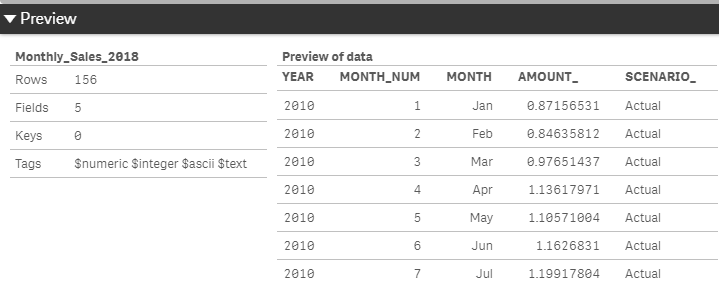
My row is Year; (2018,2017,2016...)
My columns are Month(Jan,Feb...) and Scenario_(Actual,Plan)
My measure is sum of Amount_
Data sample is below:
What I want is, Amount_ values should be cumulatively summed in pivot table for the months.
For example: March 2016 sales values should be sum of Jan 2016 and Feb 2016 on pivot table and rest of them also should be the same.
I have tried "=RangeSum(Above(Sum(AMOUNT_), 0, RowNo()))" but it did not work.
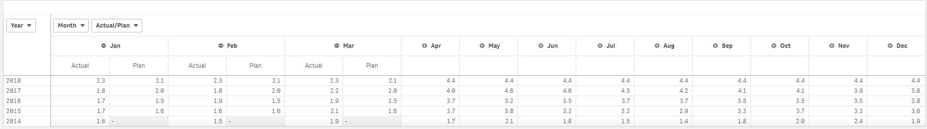
For now, I have below pivot table.
Please suggest me any solution if anyone of you gone through the same problem. Any help will be appreciated.
Thanks.
OY
- Mark as New
- Bookmark
- Subscribe
- Mute
- Subscribe to RSS Feed
- Permalink
- Report Inappropriate Content
Hi,
your expression is correct.
can you attach sample data ? the QVF ?
- Mark as New
- Bookmark
- Subscribe
- Mute
- Subscribe to RSS Feed
- Permalink
- Report Inappropriate Content
Hi,
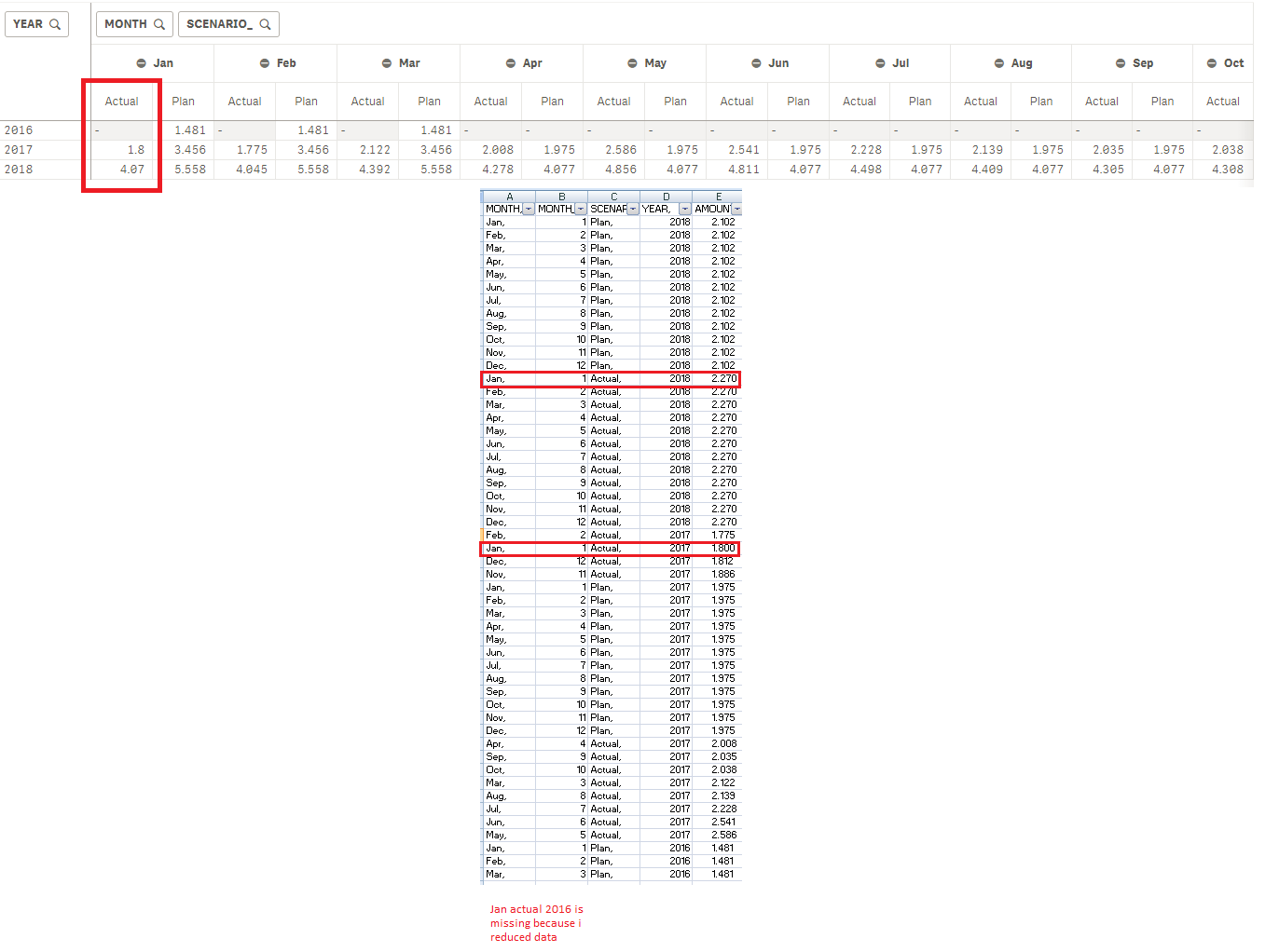
result of "=RangeSum(Above(Sum({1}AMOUNT_), 0, RowNo()))" is below, it is not what I want.
sample data:
| MONTH | MONTH_NUM | SCENARIO_ | YEAR | AMOUNT_ |
| Jan | 1 | Plan | 2018 | 2.102 |
| Feb | 2 | Plan | 2018 | 2.102 |
| Mar | 3 | Plan | 2018 | 2.102 |
| Apr | 4 | Plan | 2018 | 2.102 |
| May | 5 | Plan | 2018 | 2.102 |
| Jun | 6 | Plan | 2018 | 2.102 |
| Jul | 7 | Plan | 2018 | 2.102 |
| Aug | 8 | Plan | 2018 | 2.102 |
| Sep | 9 | Plan | 2018 | 2.102 |
| Oct | 10 | Plan | 2018 | 2.102 |
| Nov | 11 | Plan | 2018 | 2.102 |
| Dec | 12 | Plan | 2018 | 2.102 |
| Jan | 1 | Actual | 2018 | 2.270 |
| Feb | 2 | Actual | 2018 | 2.270 |
| Mar | 3 | Actual | 2018 | 2.270 |
| Apr | 4 | Actual | 2018 | 2.270 |
| May | 5 | Actual | 2018 | 2.270 |
| Jun | 6 | Actual | 2018 | 2.270 |
| Jul | 7 | Actual | 2018 | 2.270 |
| Aug | 8 | Actual | 2018 | 2.270 |
| Sep | 9 | Actual | 2018 | 2.270 |
| Oct | 10 | Actual | 2018 | 2.270 |
| Nov | 11 | Actual | 2018 | 2.270 |
| Dec | 12 | Actual | 2018 | 2.270 |
| Feb | 2 | Actual | 2017 | 1.775 |
| Jan | 1 | Actual | 2017 | 1.800 |
| Dec | 12 | Actual | 2017 | 1.812 |
| Nov | 11 | Actual | 2017 | 1.886 |
| Jan | 1 | Plan | 2017 | 1.975 |
| Feb | 2 | Plan | 2017 | 1.975 |
| Mar | 3 | Plan | 2017 | 1.975 |
| Apr | 4 | Plan | 2017 | 1.975 |
| May | 5 | Plan | 2017 | 1.975 |
| Jun | 6 | Plan | 2017 | 1.975 |
| Jul | 7 | Plan | 2017 | 1.975 |
| Aug | 8 | Plan | 2017 | 1.975 |
| Sep | 9 | Plan | 2017 | 1.975 |
| Oct | 10 | Plan | 2017 | 1.975 |
| Nov | 11 | Plan | 2017 | 1.975 |
| Dec | 12 | Plan | 2017 | 1.975 |
| Apr | 4 | Actual | 2017 | 2.008 |
| Sep | 9 | Actual | 2017 | 2.035 |
| Oct | 10 | Actual | 2017 | 2.038 |
| Mar | 3 | Actual | 2017 | 2.122 |
| Aug | 8 | Actual | 2017 | 2.139 |
| Jul | 7 | Actual | 2017 | 2.228 |
| Jun | 6 | Actual | 2017 | 2.541 |
| May | 5 | Actual | 2017 | 2.586 |
| Jan | 1 | Plan | 2016 | 1.481 |
| Feb | 2 | Plan | 2016 | 1.481 |
| Mar | 3 | Plan | 2016 | 1.481 |
| Apr | 4 | Plan | 2016 | 1.481 |
| May | 5 | Plan | 2016 | 1.481 |
| Jun | 6 | Plan | 2016 | 1.481 |
| Jul | 7 | Plan | 2016 | 1.481 |
| Aug | 8 | Plan | 2016 | 1.481 |
| Sep | 9 | Plan | 2016 | 1.481 |
| Oct | 10 | Plan | 2016 | 1.481 |
| Nov | 11 | Plan | 2016 | 1.481 |
| Dec | 12 | Plan | 2016 | 1.481 |
| May | 5 | Actual | 2016 | 1.681 |
| Jan | 1 | Actual | 2016 | 1.686 |
| Feb | 2 | Actual | 2016 | 1.829 |
| Mar | 3 | Actual | 2016 | 1.902 |
| Sep | 9 | Actual | 2016 | 1.929 |
| Oct | 10 | Actual | 2016 | 1.946 |
| Nov | 11 | Actual | 2016 | 1.949 |
| Jun | 6 | Actual | 2016 | 1.999 |
| Aug | 8 | Actual | 2016 | 2.130 |
| Apr | 4 | Actual | 2016 | 2.147 |
| Jul | 7 | Actual | 2016 | 2.194 |
| Dec | 12 | Actual | 2016 | 2.311 |
| Aug | 8 | Actual | 2015 | 1.237 |
| Jul | 7 | Actual | 2015 | 1.539 |
| Jun | 6 | Actual | 2015 | 1.550 |
| Jan | 1 | Plan | 2015 | 1.584 |
| Feb | 2 | Plan | 2015 | 1.584 |
| Mar | 3 | Plan | 2015 | 1.584 |
| Apr | 4 | Plan | 2015 | 1.584 |
| May | 5 | Plan | 2015 | 1.584 |
| Jun | 6 | Plan | 2015 | 1.584 |
| Jul | 7 | Plan | 2015 | 1.584 |
| Aug | 8 | Plan | 2015 | 1.584 |
| Sep | 9 | Plan | 2015 | 1.584 |
| Oct | 10 | Plan | 2015 | 1.584 |
| Nov | 11 | Plan | 2015 | 1.584 |
| Dec | 12 | Plan | 2015 | 1.584 |
| Feb | 2 | Actual | 2015 | 1.616 |
| Sep | 9 | Actual | 2015 | 1.693 |
| Jan | 1 | Actual | 2015 | 1.716 |
| Nov | 11 | Actual | 2015 | 1.721 |
| Dec | 12 | Actual | 2015 | 1.977 |
| Apr | 4 | Actual | 2015 | 2.057 |
| Mar | 3 | Actual | 2015 | 2.063 |
| Oct | 10 | Actual | 2015 | 2.088 |
| May | 5 | Actual | 2015 | 2.196 |
regards;
OY.
- Mark as New
- Bookmark
- Subscribe
- Mute
- Subscribe to RSS Feed
- Permalink
- Report Inappropriate Content
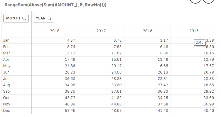
here I applied your expression with your data and it seems good.
I think your problem is related to the type of sorting of the field Year (asc/desc).
If you put the sorting of the year on descending, it will start to calculate the range from the latest year.
you need maybe to put the sorting on ascending ?
- Mark as New
- Bookmark
- Subscribe
- Mute
- Subscribe to RSS Feed
- Permalink
- Report Inappropriate Content
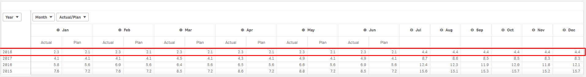
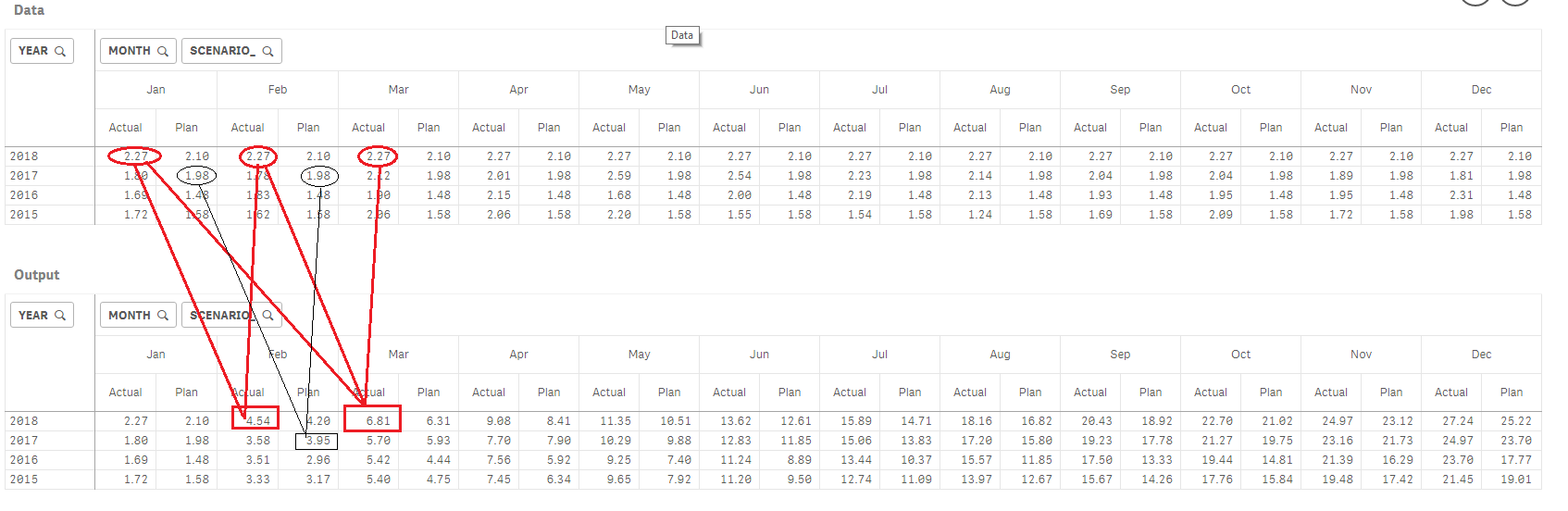
Hi, I think I have fixed it, I have add one more measure
now two measures like below:
for Actuals:
sum({<MONTH={"<=$(=max(MONTH))"}>}aggr(rangesum(above(Sum({<MONTH=,YEAR=,SCENARIO_={'Actual'}>}AMOUNT_),0,RowNo())),YEAR,(MONTH,(num))))
for plans:
sum({<MONTH={"<=$(=max(MONTH))"}>}aggr(rangesum(above(Sum({<MONTH=,YEAR=,SCENARIO_={'Plan'}>}AMOUNT_),0,RowNo())),YEAR,(MONTH,(num))))
result is below: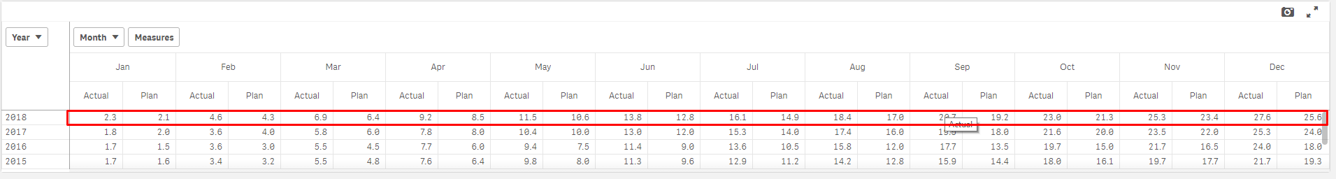
- Mark as New
- Bookmark
- Subscribe
- Mute
- Subscribe to RSS Feed
- Permalink
- Report Inappropriate Content
I don't see here the cumulative values related to your data structure and values.. but if the problem is solved for you don't hesitate to close the thread 
- Mark as New
- Bookmark
- Subscribe
- Mute
- Subscribe to RSS Feed
- Permalink
- Report Inappropriate Content
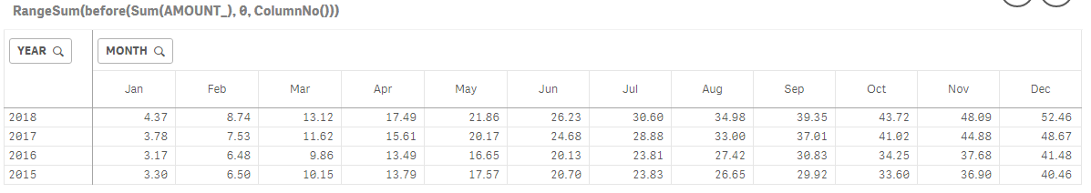
Hi Onur,
You just need to use RangeSum(Before(Sum(AMOUNT_), 0, ColumnNo())) as measure on your pivot table. If you want to get running sum on horizantal, you have to use Before() instead of Above() and ColumnNo() instead of RowNo(). Above() and RowNo() can be used for vertical running sums.
For example: March 2016 sales values should be sum of Jan 2016 and Feb 2016 on pivot table and rest of them also should be the same.
I am not pretty sure about your actual need but if you want to show sum of Jan and Feb on Mar Column (except Mar value). you need to
edit this expression.
RangeSum(Before(Sum(AMOUNT_), 1, ColumnNo()))
Hope it helps,
Kaan ERİŞEN
- Mark as New
- Bookmark
- Subscribe
- Mute
- Subscribe to RSS Feed
- Permalink
- Report Inappropriate Content
Hi Kaan;
Thank you for your kind help.
Your code is working if the year values are in columns.
For my case, month values should be in colomn and year values should be in row.
Provided code 'RangeSum(Before(Sum(AMOUNT_), 0, ColumnNo())) ' not working for this case.
regards;
Onur
- Mark as New
- Bookmark
- Subscribe
- Mute
- Subscribe to RSS Feed
- Permalink
- Report Inappropriate Content
How about this?
Measure : sum(aggr(rangesum(above(Sum(AMOUNT_),0,RowNo())),SCENARIO_,YEAR,MONTH))
- Mark as New
- Bookmark
- Subscribe
- Mute
- Subscribe to RSS Feed
- Permalink
- Report Inappropriate Content
Hi,
RangeSum(Sum(Amount_), Before(TOTAL Sum(Amount_), 1, ColumnNo(TOTAL)))
or
In any case, someone needs to use a set analysis
=rangesum(sum ({$<Column={"Value"}>}Amount_ ) , Before(TOTAL sum ({$<Column={"Value"}>}Amount_ ) ,1 , ColumnNo(TOTAL)))