Unlock a world of possibilities! Login now and discover the exclusive benefits awaiting you.
- Qlik Community
- :
- Forums
- :
- Analytics
- :
- New to Qlik Analytics
- :
- ABC Analysis w. 2 dimensions
- Subscribe to RSS Feed
- Mark Topic as New
- Mark Topic as Read
- Float this Topic for Current User
- Bookmark
- Subscribe
- Mute
- Printer Friendly Page
- Mark as New
- Bookmark
- Subscribe
- Mute
- Subscribe to RSS Feed
- Permalink
- Report Inappropriate Content
ABC Analysis w. 2 dimensions
Hi
Im attempting to do an ABC analysis by customer by product in QlikSense. The end result is to categorize and label each product as one of the following
A – (represents 50% of customer usage)
B – (represents 30% of customer usage)
C – (represents 20% of customer usage)
we have dimensions of
CustomerId
ProductID
and have been using Shipqty as a measure
we've studied Recipe for an ABC Analysis, Pareto on 2 dimensions among others....
Our last try was:
=Aggr(if(rangesum(Above(sum(ShipQty)/sum(TOTAL <CustomerID> ShipQty),0,rowno() ))>=0.50,'A',if(rangesum(Above(sum(ShipQty)/sum
(TOTAL <CustomerID> ShipQty),0,rowno()))>=0.30,'B','C')),CustomerID,(ProductID,(=Sum(ShipQty))))
Any help to rework the above calculated dimension to get our end result would be much appreciated
below is an example of the end result data
| CustomerID | ProductID | Rank | Total Usage |
| 106837 | 10111255 | A | 48 |
| 106837 | 10111256 | A | 27 |
| 106837 | 10111257 | A | 27 |
| 106837 | 10111258 | A | 27 |
| 106837 | 10111259 | C | 24 |
| 106837 | 10111260 | C | 24 |
| 106837 | 10111261 | C | 20 |
| 106837 | 10111262 | A | 20 |
| 106837 | 10111263 | A | 12 |
| 106837 | 10111264 | A | 10 |
| 106837 | 10111265 | B | 10 |
| 106837 | 10111266 | B | 10 |
| 106837 | 10111267 | C | 6 |
| 106837 | 10111268 | A | 6 |
| 106837 | 10111269 | B | 6 |
| 106837 | 10111270 | B | 6 |
| 106837 | 10111271 | C | 4 |
| 106837 | 10111272 | C | 4 |
| 106837 | 10111273 | B | 4 |
| 106837 | 10111274 | C | 2 |
| 106837 | 10111275 | C | 1 |
| 106837 | 10111276 | C | 1 |
| 106837 | 10111277 | C | 1 |
| 106950 | 10111278 | A | 12 |
| 106950 | 10111279 | A | 8 |
| 106950 | 10111280 | B | 8 |
| 106950 | 10111281 | A | 7 |
| 106950 | 10111282 | B | 6 |
| 106950 | 10111283 | A | 5 |
| 106950 | 10111284 | C | 4 |
| 106950 | 10111285 | C | 4 |
| 106950 | 10111286 | A | 4 |
| 106950 | 10111287 | A | 4 |
| 106950 | 10111288 | C | 3 |
| 106950 | 10111289 | C | 3 |
| 106950 | 10111290 | A | 3 |
| 106950 | 10111291 | C | 2 |
| 106950 | 10111292 | C | 2 |
| 106950 | 10111293 | C | 1 |
| 106950 | 10111294 | A | 1 |
| 106950 | 10111295 | A | 1 |
| 106950 | 10111296 | A | 1 |
Thanks
Andrew
- « Previous Replies
-
- 1
- 2
- Next Replies »
- Mark as New
- Bookmark
- Subscribe
- Mute
- Subscribe to RSS Feed
- Permalink
- Report Inappropriate Content
Not sure what is wrong, but it seems that you are missing a little part of the syntax
=Aggr(
If(RangeSum(Above(Sum(ShipQty)/Sum(TOTAL <CustomerID> ShipQty), 0, RowNo())) >= 0.50, 'A',
If(RangeSum(Above(Sum(ShipQty)/Sum(TOTAL <CustomerID> ShipQty), 0, RowNo())) >= 0.30, 'B', 'C')), CustomerID, (ProductID, (=Sum(ShipQty), DESC)))
- Mark as New
- Bookmark
- Subscribe
- Mute
- Subscribe to RSS Feed
- Permalink
- Report Inappropriate Content
Thanks Sunny
appreciate your help and added the syntax, but its still not calculating correctly
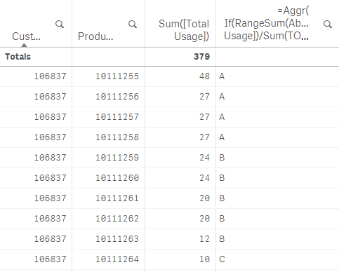
To help illustrate, we pulled the table below and included customer, product, usage and the Rank it populated
our end game is to have the products representing up to the first 50% of usage(products 10111255-10111258) to have an A designation
products (10111259-10111262) should have a B designation and the remainder a C
However, in the sample below the top usage items calculated with A,B and C ratings
| CustomerID | ProductID | RANK | Total Usage |
| 106837 | 10111255 | A | 48 |
| 106837 | 10111256 | B | 27 |
| 106837 | 10111257 | C | 27 |
| 106837 | 10111258 | C | 27 |
| 106837 | 10111259 | A | 24 |
| 106837 | 10111260 | A | 24 |
| 106837 | 10111261 | A | 20 |
| 106837 | 10111262 | B | 20 |
| 106837 | 10111263 | C | 12 |
| 106837 | 10111264 | A | 10 |
| 106837 | 10111265 | A | 10 |
| 106837 | 10111266 | B | 10 |
| 106837 | 10111267 | A | 6 |
| 106837 | 10111268 | A | 6 |
| 106837 | 10111269 | A | 6 |
| 106837 | 10111270 | B | 6 |
| 106837 | 10111271 | A | 4 |
| 106837 | 10111272 | A | 4 |
| 106837 | 10111273 | A | 4 |
| 106837 | 10111274 | A | 2 |
| 106837 | 10111275 | A | 1 |
| 106837 | 10111276 | A | 1 |
| 106837 | 10111277 | A | 1 |
- Mark as New
- Bookmark
- Subscribe
- Mute
- Subscribe to RSS Feed
- Permalink
- Report Inappropriate Content
Would you be able to share a sample to see the issue?
- Mark as New
- Bookmark
- Subscribe
- Mute
- Subscribe to RSS Feed
- Permalink
- Report Inappropriate Content
Sure thing. but, can you please forward a link on how to attach a sample document in the format you need (still very new to qlik sense)
- Mark as New
- Bookmark
- Subscribe
- Mute
- Subscribe to RSS Feed
- Permalink
- Report Inappropriate Content
- Mark as New
- Bookmark
- Subscribe
- Mute
- Subscribe to RSS Feed
- Permalink
- Report Inappropriate Content
Thanks Sunny - please see attached
- Mark as New
- Bookmark
- Subscribe
- Mute
- Subscribe to RSS Feed
- Permalink
- Report Inappropriate Content
This seems like an already aggregated data, right? I was looking for some raw data or the qvw file where you might have been trying this.
- Mark as New
- Bookmark
- Subscribe
- Mute
- Subscribe to RSS Feed
- Permalink
- Report Inappropriate Content
Hi Andrew,
I did a small adjustment and got results similar to your expectations:
=Aggr(
If(RangeSum(Above(Sum(ShipQty)/Sum(TOTAL <CustomerID> ShipQty), 0, RowNo())) <= 0.50, 'A',
If(RangeSum(Above(Sum(ShipQty)/Sum(TOTAL <CustomerID> ShipQty), 0, RowNo())) <= 0.80, 'B', 'C')), CustomerID, (ProductID, (=Sum(ShipQty), DESC)))
Hope this helps.
Juraj
- Mark as New
- Bookmark
- Subscribe
- Mute
- Subscribe to RSS Feed
- Permalink
- Report Inappropriate Content
Thanks Sunny - please see attached.
- « Previous Replies
-
- 1
- 2
- Next Replies »