Conditional Color R,Y,G based on % Change

[blakeB]

Using the below formula to show red or green based off previous month's conversion rate (table reference).

=If(above(sum({<Month={'$(=max(Month))'}>} [Overall Conversion Rate])) > sum({<Month={'$(=max(Month))'}>} [Overall Conversion Rate]), red(), green())

Not sure how to improve this expression to red, yellow, green based off threshold. For example, if previous month conversion was less than 1% change up or down I'd like it to show yellow.

Any insights or help would be great.

Thanks

[vvira1316]

Will you be able to share a sample app with mock data so we can understand what challenge you are running into

[blakeB]

Climber KPI with red/green formulaKPI disappears when you add the red,yellow,green string

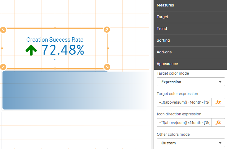
Below is a table from excel with mock figures (along with screenshots from the dashboard above) that I am pulling into Qlik. Not sure how to attach a mock app, so hopefully this helps. The current formula for green or red, is as follows:

=If(above(sum({<Month={'$(=max(Month))'}>} [Overall Conversion Rate])) > sum({<Month={'$(=max(Month))'}>} [Overall Conversion Rate]), red(), green())

Seems to work on my end, but I've tried all the recommended suggestions on this thread and can't seem to get red/yellow/green.

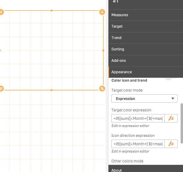
When I use the red/yellow/green formula the KPI visual disapears (See attached above). Formula:

=If((sum({<Month={'$(=max(Month))'}>} [Overall Conversion Rate]) - above(sum({<Month={'$(=max(Month))'}>} [Overall Conversion Rate])))<0.1
 and (sum({<Month={'$(=max(Month))'}>} [Overall Conversion Rate]) - above(sum({<Month={'$(=max(Month))'}>} [Overall Conversion Rate]))) >= -0.1, Yellow(),
 If((sum({<Month={'$(=max(Month))'}>} [Overall Conversion Rate]) - above(sum({<Month={'$(=max(Month))'}>} [Overall Conversion Rate])))>0.1,Green(),
  If((sum({<Month={'$(=max(Month))'}>} [Overall Conversion Rate]) - above(sum({<Month={'$(=max(Month))'}>} [Overall Conversion Rate])))<-0.1,Red())))

Month	Converison Rate
1/1/2018	0.7246
2/1/2018	0.7395
3/1/2018	0.7318
4/1/2018	0.7213
5/1/2018	0.7238
6/1/2018	0.7223
7/1/2018	0.7203
8/1/2018	0.7183
9/1/2018	0.7163
10/1/2018	0.7143

[blakeB]

When I input the formula you provided, once I apply and save, if I leave the sheet and come back the KPI is showing blank...see below. Thanks

[timpoismans]

When replying, you can attach files, for Qlik Sense apps, you'll need to zip them first as we can't upload .qvf at the moment.

That said, where does the field [Overall Conversion Rate]? How is it calculated? 

Having a mock app would help us a lot though, so we are in the exact same situation you are when encountering the issue.

[vvira1316]

=If((sum({<Month={'$(=max(Month))'}>} [Overall Conversion Rate]) - above(sum({<Month={'$(=max(Month))'}>} [Overall Conversion Rate])))< <=0.1
 and (sum({<Month={'$(=max(Month))'}>} [Overall Conversion Rate]) - above(sum({<Month={'$(=max(Month))'}>} [Overall Conversion Rate]))) >= -0.1, Yellow(),
 If((sum({<Month={'$(=max(Month))'}>} [Overall Conversion Rate]) - above(sum({<Month={'$(=max(Month))'}>} [Overall Conversion Rate])))>0.1,Green(),
  If((sum({<Month={'$(=max(Month))'}>} [Overall Conversion Rate]) - above(sum({<Month={'$(=max(Month))'}>} [Overall Conversion Rate])))<-0.1,Red())))

I think here it should have been <= rather than just < because any value above 0.1 will be green, any value less than -0.1 will be red and any value between (including) -0.1 and 0.1 should be represented with yellow

I'm working with sample you have provided to give you a working solution but in the mean time you can try above change. In the sample you have provided the delta is always much smaller than 0.1 (+/-) and value itself is 0.7nnn

Please advise on data

[blakeB]

Thanks for your help. I changed the formaul to show <= but the KPI is still blank, and in regards to the data I utilize 0.7nnn because I display it as a %. Using 0.1 (+/-) I can always change to 0.05 for this particular excercise. Once I figure out how to get the red/yellow/green working I'm going to adapt the expression to all of the KPIs. You can use 0.05 to help solve the problem.

Thanks again and I will keep an eye out for the working solution you mentioned.

[vvira1316]

Hi,

NoConcatenate
[ConvInfo]:
LOAD
Date("Month", 'MM/DD/YYYY') as ConvRateDate,
Dual(Year(Date("Month", 'MM/DD/YYYY'))&'-'&Month(Date("Month", 'MM/DD/YYYY')), monthstart(Date("Month", 'MM/DD/YYYY'))) AS [Conv YearMonth],
"Converison Rate",
"Converison Rate Diff"
FROM [lib:/NumTest.xlsx]
(ooxml, embedded labels, table is Sheet1);

Expression 

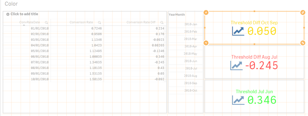
=If((Sum({<[Conv YearMonth]={"2018-Oct"}>} [Converison Rate]) - Sum({<[Conv YearMonth]={"2018-Sep"}>} [Converison Rate])) <= 0.1
and (Sum({<[Conv YearMonth]={"2018-Oct"}>} [Converison Rate]) - Sum({<[Conv YearMonth]={"2018-Sep"}>} [Converison Rate])) >= -0.1, RGB(250, 220, 0),
If((Sum({<[Conv YearMonth]={"2018-Oct"}>} [Converison Rate]) - Sum({<[Conv YearMonth]={"2018-Sep"}>} [Converison Rate])) > 0.1, RGB(0, 255, 0), RGB(255, 0, 0)))

I hope this helps.

[blakeB]

Thanks! I was hoping to change the actual trend icon, but will try to apply the above expression to the icon conditioning. Assuming that it will likely work the same.

[vvira1316]

I hope you were able to successfully change the expression and use it conditionally with the ICON. Advise if you have any further challenges