How to show top 3 value based on second dimension in 100 % stacked bar chart

[Rajkumar]

Hi All,

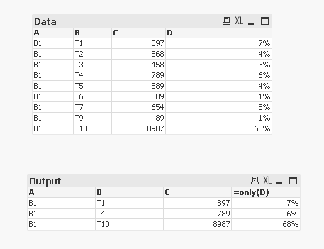
How to show top 3 value based on second dimension in 100 % stacked bar chart.

Input :

A    B        C          D
B1 T10 8987 68%
B1 T1 897 7%
B1 T4 789 6%
B1 T7 654 5%
B1 T5 589 4%
B1 T2 568 4%
B1 T3 458 3%
B1 T6 89 1%
B1 T9 89 1%

OUTPUT:

A     B        C
B1 T10 68%
B1 T1 7%
B1 T4 6%

[Taoufiq_Zarra]

Hi,

you can use the script below to replace the A field in dimension

=aggr(if( rank(Only(D),4)<=3,A), ID)

you can get results like:

the load script:

Data:
load Rowno() as ID,* inline [
A,B,C,D
B1,T10,8987,68%
B1,T1,897,7%
B1,T4,789,6%
B1,T7,654,5%
B1,T5,589,4%
B1,T2,568,4%
B1,T3,458,3%
B1,T6,89,1%
B1,T9,89,1%
];

this script  also works without ID on load

=aggr(if( rank(Only(D),4)<=3,A), B)

[Rajkumar]

Can you help on to do  3 column instead of 4 column to achieve same output . Ex similiar % column like 4 

B1  T10 8987 10673 84.2%
B1  T1  897  10673 8.4%
B1  T4  789  10673 7.4%

[Taoufiq_Zarra]

I'm sorry, but I didn't really understand your request

[Rajkumar]

Hi,

This is my desired Output.

A      B         C       D          E 

B1  T10 8987 10673 84.2%
B1  T1  897  10673 8.4%
B1  T4  789  10673 7.4%

[Taoufiq_Zarra]

I still don't get it.

How do you get from this input

Input :

A B C D
B1 T10 8987 68%
B1 T1 897 7%
B1 T4 789 6%
B1 T7 654 5%
B1 T5 589 4%
B1 T2 568 4%
B1 T3 458 3%
B1 T6 89 1%
B1 T9 89 1%

 this output :

A B C D E

B1 T10 8987 10673 84.2%
B1 T1 897 10673 8.4%
B1 T4 789 10673 7.4%

For example 10673 ? or 84.2% ?

[Rajkumar]

10673 is the sum of three values 8987 + 897  +  789 
&

 84.2% is 8987/10673

[Taoufiq_Zarra]

Ah , I get it now., like :

to get E and F use this script

for E:

=sum(total aggr(if( rank(Only(D),4)<=3,C), B))

for F:

=num(C/sum(total aggr(if( rank(Only(D),4)<=3,C), B)),'###0,00%')

[Kushal_Chawda]

Above solution may not work if you have multiple values in A field like below

A,B,C
B1,T10,8987
B1,T1,897
B1,T4,789
B1,T7,654
B1,T5,589
B1,T2,568
B1,T3,458
B1,T6,89
B1,T9,89
B2,T1,100
B2,T11,250
B2,T3,300
B2,T4,400

This will make chart expression more complex. Hence, providing script solution

T1:
load * inline [
A,B,C
B1,T10,8987
B1,T1,897
B1,T4,789
B1,T7,654
B1,T5,589
B1,T2,568
B1,T3,458
B1,T6,89
B1,T9,89
B2,T1,100
B2,T11,250
B2,T3,300
B2,T4,400
];

left join(T1)
Load A,
B,
AutoNumber(Sum(C),A) as Rank
Resident T1
Group by A,B
Order by C desc;

Left Join(T1)
Load A,
Sum(C) as D
Resident T1
where Rank<=3
Group by A;

Now create Chart,

Dimension

A,

B

Expression:

C -

=Sum({<Rank={"<=3"}>}C)

D-

=Sum({<Rank={"<=3"}>}D)

E-

=Sum({<Rank={"<=3"}>}C)/Sum({<Rank={"<=3"}>}D)