Unlock a world of possibilities! Login now and discover the exclusive benefits awaiting you.
- Qlik Community
- :
- Forums
- :
- Analytics
- :
- New to Qlik Analytics
- :
- Pivot Table - Adding a %
- Subscribe to RSS Feed
- Mark Topic as New
- Mark Topic as Read
- Float this Topic for Current User
- Bookmark
- Subscribe
- Mute
- Printer Friendly Page
- Mark as New
- Bookmark
- Subscribe
- Mute
- Subscribe to RSS Feed
- Permalink
- Report Inappropriate Content
Pivot Table - Adding a %
Hiya,
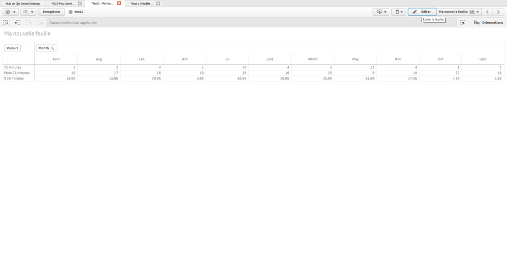
I've created a Qlik Sense Dashboard and used a pivot table in this to show how many times people have clocked 25 minutes or less and how many have clocked more than 25 minutes.
I would then like to be able to show a % that were less than 25 minutes. Ideally I don't want my pivot table to have a total line (because it shows it at the top and I don't want that).
I've tried so many ways to try to get this to work, but I can't seem to... I've attached an excel version of what I want it to show, so please could someone try to help!! Nothing I've tried is working!!
Many Thanks in Advance!!
Megan
- Tags:
- pivot
- pivot table
Accepted Solutions
- Mark as New
- Bookmark
- Subscribe
- Mute
- Subscribe to RSS Feed
- Permalink
- Report Inappropriate Content
To do this, I changed each of my rows and made them measures with the formulas:
25 Mins - =count({<[Time Check]={'25Min'}>}[Employee Name + Date])
Ok - =count({<[Time Check]={'OK'}>}[Employee Name + Date])
% Over 25 Mins - =(count({<[Time Check]={'25Min'}>}[Employee Name + Date]))/count([Employee Name + Date])
Then formatted the % one to Number and % and made the rows measures.
- Mark as New
- Bookmark
- Subscribe
- Mute
- Subscribe to RSS Feed
- Permalink
- Report Inappropriate Content
hello,
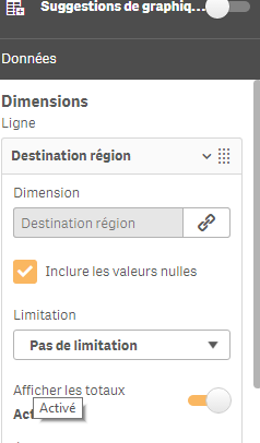
delete the option :
show totals
after create a measure :
sum(clock less 25)/(sum(clock less 25)+sum(clock more 25))
where clock less 25 is your field clocked 25 minutes or less ans clock more 25 is clocked more than 25 minutes
or column(1)/(column(1)/column(2))
bye
- Mark as New
- Bookmark
- Subscribe
- Mute
- Subscribe to RSS Feed
- Permalink
- Report Inappropriate Content
This doesn't seem to be giving me what I want. It's adding it as another column and giving me no figures. I want it at the bottom for each month the same way the data of less than 25 minutes and more than are.
Thanks
- Mark as New
- Bookmark
- Subscribe
- Mute
- Subscribe to RSS Feed
- Permalink
- Report Inappropriate Content
like that right? see the attached file
- Mark as New
- Bookmark
- Subscribe
- Mute
- Subscribe to RSS Feed
- Permalink
- Report Inappropriate Content
That's not what mine was looking like, but that is what I would like it to show... Here is your formula, trying to replicate it doesn't like the 'Data', what part is that referring to? Is that the file name that was uploaded or something?
Sum({<F1={'25 Minutes'}>} Data)/(Sum({<F1={'25 Minutes'}>} Data)+Sum({<F1={'More than 25 Minutes'}>} Data))
- Mark as New
- Bookmark
- Subscribe
- Mute
- Subscribe to RSS Feed
- Permalink
- Report Inappropriate Content
if you see the script , you can watch i create a file with data and i make a crosstable to pivot the table.
for you replace data by your measure and F1 by your dimension.
to finish, replace 25 minutes and more 25 minutes by value of dimension
on the graphic, leave the dimension which contains 25 minutes and more 25 minutes
if it's not clear for you, can you put a screenshot of your model or script and i give you the good expression
- Mark as New
- Bookmark
- Subscribe
- Mute
- Subscribe to RSS Feed
- Permalink
- Report Inappropriate Content
To do this, I changed each of my rows and made them measures with the formulas:
25 Mins - =count({<[Time Check]={'25Min'}>}[Employee Name + Date])
Ok - =count({<[Time Check]={'OK'}>}[Employee Name + Date])
% Over 25 Mins - =(count({<[Time Check]={'25Min'}>}[Employee Name + Date]))/count([Employee Name + Date])
Then formatted the % one to Number and % and made the rows measures.

