Solved: Aggregate Rank() on a field - Qlik Community

qlikwiz123 · ‎2019-05-16

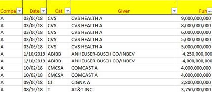
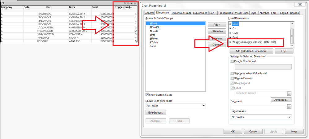
Please look at the screenshot below.

I just sorted on Funds from Highest to lowest and since CVS HEALTH has the highest Funds overall, the Rank for all CVS from 'Giver' column should be 1.

Then all rows with 'Giver' - ANHEUSER-BUSCH CO/INBEV should be 2, COMCAST A should be 3 and so on...

Nicole-Smith · ‎2019-05-17

So it sounds like you want max() instead of sum()?

Using the following as a dimension:
=Aggr(Rank(aggr(max(Funds),Cat), 1, 1),Cat)

Results in this:

Cat	Company	Date	Giver	Funds	max(total <Cat> Funds)	=Aggr(Rank(aggr(max(Funds),Cat), 1, 1),Cat)
CVS	A	3/6/2018	CVS HEALTH A	9000000000	9000000000	1
CVS	A	3/6/2018	CVS HEALTH A	8000000000	9000000000	1
CVS	A	3/6/2018	CVS HEALTH A	6000000000	9000000000	1
CVS	A	3/6/2018	CVS HEALTH A	5000000000	9000000000	1
CVS	A	3/6/2018	CVS HEALTH A	3000000000	9000000000	1
CVS	A	3/6/2018	CVS HEALTH A	2000000000	9000000000	1
CVS	A	3/6/2018	CVS HEALTH A	1000000000	9000000000	1
ABIBB	A	3/20/2018	ANHEUSER-BUSCH INBEV WOR	2500000000	4250000000	2
ABIBB	A	3/20/2018	ANHEUSER-BUSCH INBEV WOR	1500000000	4250000000	2
ABIBB	A	3/20/2018	ANHEUSER-BUSCH INBEV WOR	500000000	4250000000	2
ABIBB	A	1/10/2019	ANHEUSER-BUSCH CO/INBEV	4250000000	4250000000	2
ABIBB	A	1/10/2019	ANHEUSER-BUSCH CO/INBEV	4000000000	4250000000	2
ABIBB	A	1/10/2019	ANHEUSER-BUSCH CO/INBEV	2500000000	4250000000	2
ABIBB	A	1/10/2019	ANHEUSER-BUSCH CO/INBEV	2000000000	4250000000	2
ABIBB	A	1/10/2019	ANHEUSER-BUSCH CO/INBEV	750000000	4250000000	2
CMCSA	A	2/1/2018	COMCAST A	1200000000	4000000000	3
CMCSA	A	2/1/2018	COMCAST A	1000000000	4000000000	3
CMCSA	A	10/2/2018	COMCAST A	4000000000	4000000000	3
CMCSA	A	10/2/2018	COMCAST A	3000000000	4000000000	3
CMCSA	A	10/2/2018	COMCAST A	2500000000	4000000000	3
CMCSA	A	10/2/2018	COMCAST A	2000000000	4000000000	3
CMCSA	A	10/2/2018	COMCAST A	1750000000	4000000000	3
CMCSA	A	10/2/2018	COMCAST A	1500000000	4000000000	3
CMCSA	A	10/2/2018	COMCAST A	1250000000	4000000000	3
CMCSA	A	10/2/2018	COMCAST A	1000000000	4000000000	3
CMCSA	A	10/2/2018	COMCAST A	500000000	4000000000	3
CI	A	9/6/2018	CIGNA A	3800000000	3800000000	4
CI	A	9/6/2018	CIGNA A	3100000000	3800000000	4
CI	A	9/6/2018	CIGNA A	3000000000	3800000000	4
CI	A	9/6/2018	CIGNA A	2200000000	3800000000	4
CI	A	9/6/2018	CIGNA A	1750000000	3800000000	4
CI	A	9/6/2018	CIGNA A	1250000000	3800000000	4
CI	A	9/6/2018	CIGNA A	1000000000	3800000000	4
CI	A	9/6/2018	CIGNA A	700000000	3800000000	4

Also attaching the example file with this change.

View solution in original post

Nicole-Smith · ‎2019-05-16

The following works as a dimension:

qlikwiz123 · ‎2019-05-16

@Nicole-Smith

Hi,

Please find the Attached QVW. The same is not working on my end.

Nicole-Smith · ‎2019-05-16

It's working properly based on the sum of Funds per Cat (I've updated the chart in your example file to contain the sum of Funds by Cat as an expression).

Do you maybe want it grouped by Giver instead of Cat? I've added a second chart that does that.

qlikwiz123 · ‎2019-05-16

@Nicole-Smith Thanks you so much. Let me check this one

qlikwiz123 · ‎2019-05-16

qlikwiz123 · ‎2019-05-16

@Nicole-Smith

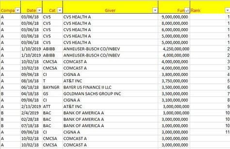
Please look at the attached Excel Source file. Here, you can clearly see that the Highest to lowest Funds with respect to Cat, the order is different. I have added a Rank column manually to help you understand how my rankings should look like.

1. How do I get them to show same rank if the Funds value is same instead of multiple numbers like below?

2. This is how my Ranks should look like, if you look at the Excel file sorted based on Funds from highest to lowest.

Nicole-Smith · ‎2019-05-16

If grouping by Cat, JPM totals to more than CVS (as seen in the first chart in my previous example file--second to last column). I'm not sure what your Excel file is doing to ignore JPM. From the totals on that first chart, I can see that the ranking function that I wrote is working properly.

If you want it to show the values without the dashes, you can change the extra parameters of the Rank function to fit your needs. I usually go with 1 and 1 but other options can be found here. For example:
=Aggr(Rank(aggr(Sum(Funds),Cat), 1, 1),Cat)

qlikwiz123 · ‎2019-05-17

If you look at the Excel file attached or even the screenshot, JPM is not the highest Funds, it is the CVS and then ABIBB and CMCSA and so on....

Nicole-Smith · ‎2019-05-17

You're right--the sum I have isn't working properly. If I can figure out why, I can fix this rank function...

Aggregate Rank() on a field

aggr

aggregate

Rank