Unlock a world of possibilities! Login now and discover the exclusive benefits awaiting you.
- Qlik Community
- :
- All Forums
- :
- QlikView App Dev
- :
- Re: Coloring cells according to a validation
- Subscribe to RSS Feed
- Mark Topic as New
- Mark Topic as Read
- Float this Topic for Current User
- Bookmark
- Subscribe
- Mute
- Printer Friendly Page
- Mark as New
- Bookmark
- Subscribe
- Mute
- Subscribe to RSS Feed
- Permalink
- Report Inappropriate Content
Coloring cells according to a validation
Hello,
I'm generating a table where I group for a given service, several tasks. These tasks have different priority (critical, average and low) and I need to display a color map per service.
If any task is critical, turn it red. (regardless of whether you have medium or low tasks)
If any task is average, and has no critical, its yellow
If all tasks are low, they turn green.
Example:
| Service | Task | Color |
|---|---|---|
| Service1 | Task 1: Critical Task 2: Media Task 3: Media Task 4: Low | Red |
| Service 2 | Taks 1: Low Task 2: Low Task 3: Media | Orange |
| Service 3 | Task 1: Low Task 2: Low Task 3: Low | Green |
thank you very much!
- « Previous Replies
-
- 1
- 2
- Next Replies »
Accepted Solutions
- Mark as New
- Bookmark
- Subscribe
- Mute
- Subscribe to RSS Feed
- Permalink
- Report Inappropriate Content
Hi Paola,
You can use
=Pick(Wildmatch(Concat(TOTAL <Service>Task,'|'),'*Critical*','*Medium*','*Low*'),RGB(255,0,0),RGB(255,165,0),RGB(0,255,0))
to give
| Service | Task |
|---|---|
| Service 1 | Task 1:critical |
| Service 1 | Task 2:medium |
| Service 1 | Task 3:medium |
| Service 1 | Task 4:low |
| Service 2 | Task 1:low |
| Service 2 | Task 2:low |
| Service 2 | Task 3:medium |
| Service 3 | Task 1:low |
| Service 3 | Task 2:low |
| Service 3 | Task 3:low |
Regards
Andrew
- Mark as New
- Bookmark
- Subscribe
- Mute
- Subscribe to RSS Feed
- Permalink
- Report Inappropriate Content
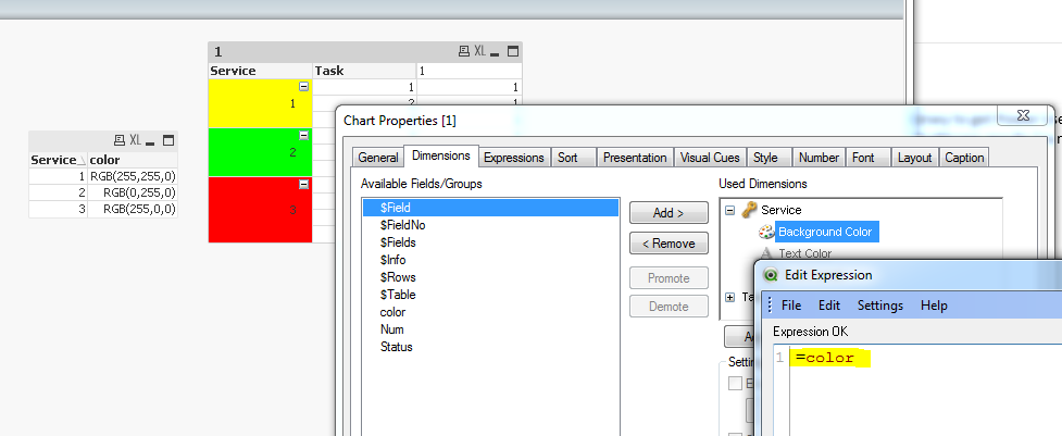
There must be a better way of implementing it but one way of doing it is to assign numbers per task status such as Critical as 3, Medium as 2 and Low as 1. In that way you can do an aggregation (max) on that number group by Service and then you can assign a color to that number.
In the script:
dat:
LOAD * Inline [
Service,Task,Status
1,1,low
1,2,low
1,3,medium
2,1,low
2,2,low
2,3,low
3,1,critical
3,2,medium
3,3,medium
3,4,low];
Join
LOAD * Inline [
Status,Num
low,1
medium,2
critical,3
];
// Each service will have a status and color
LOAD Service,if(max(Num) = 3,RGB(255,0,0),if(max(Num)=2,RGB(255,255,0),RGB(0,255,0))) as color Resident dat
Group by Service ;
Then in the UI:
- Mark as New
- Bookmark
- Subscribe
- Mute
- Subscribe to RSS Feed
- Permalink
- Report Inappropriate Content
thank you,
The colors aren't based in if there are more critical or medium, or low, the rules are:
If exist, some critical, then the color is red.
if exist some medium and some low and any critical, then the color is yellow.
If exist only lows, the the color is green
- Mark as New
- Bookmark
- Subscribe
- Mute
- Subscribe to RSS Feed
- Permalink
- Report Inappropriate Content
Hi,
It works with paste the following formula as background expression color :
=if(SubStringCount (concat(TOTAL <Service> {<Service={"Service 1"}>} Task),'critical')>0,lightred(),
if(SubStringCount (concat(TOTAL <Service> {<Service={"Service 2"}>} Task),'media')>0
and SubStringCount (concat(TOTAL <Service> {<Service={"Service 2"}>} Task),'critical')=0 ,rgb(255,156,57),
if(SubStringCount (concat(TOTAL <Service> {<Service={"Service 3"}>} Task),'low')=3,lightgreen())))
- Mark as New
- Bookmark
- Subscribe
- Mute
- Subscribe to RSS Feed
- Permalink
- Report Inappropriate Content
Hi Paola,
For each service try this expression to set the colour:
Pick(Wildmatch(Concat(Task,'|'),'*Critical*','*Medium*','*Low*'),Red().Yellow(),Green())
Regards
Andrew
- Mark as New
- Bookmark
- Subscribe
- Mute
- Subscribe to RSS Feed
- Permalink
- Report Inappropriate Content
Can you share me the document?.
Regards.
- Mark as New
- Bookmark
- Subscribe
- Mute
- Subscribe to RSS Feed
- Permalink
- Report Inappropriate Content
Of course, see attached .qvw
Regards
- Mark as New
- Bookmark
- Subscribe
- Mute
- Subscribe to RSS Feed
- Permalink
- Report Inappropriate Content
I have just surrender that you last line "If all tasks are low, they turn green." is not well taking in account in my formula because it was hard code with 3 rows.
So replace, the last line
if(SubStringCount (concat(TOTAL <Service> {<Service={"Service 3"}>} Task),'low')=3,lightgreen())))
with
if(SubStringCount (concat(TOTAL <Service> {<Service={"Service 3"}>} Task),'low')=NoOfRows(),lightgreen())))
- Mark as New
- Bookmark
- Subscribe
- Mute
- Subscribe to RSS Feed
- Permalink
- Report Inappropriate Content
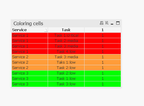
Hi Paola,
You can get
| Service | Task |
|---|---|
| Service 1 | Task 1:critical |
| Service 1 | Task 2:medium |
| Service 1 | Task 3:medium |
| Service 1 | Task 4:low |
| Service 2 | Task 1:low |
| Service 2 | Task 2:low |
| Service 2 | Task 3:medium |
| Service 3 | Task 1:low |
| Service 3 | Task 2:low |
| Service 3 | Task 3:low |
With this background colour:
=Pick(Wildmatch(Concat(TOTAL <Service>Task,'|'),'*Critical*','*Medium*','*Low*'),LightRed(),Yellow(),LightGreen())
Cheers
Andrew
- Mark as New
- Bookmark
- Subscribe
- Mute
- Subscribe to RSS Feed
- Permalink
- Report Inappropriate Content
mmm... i have the priority in other col:
| Service | Task | Priority | Color |
|---|---|---|---|
| Service1 | Task 1 Task 2 Task 3 Task 4 | Critical Media Media Low | Red |
| Service 2 | Taks 1 Task 2 Task 3 | Low Low Media | Orange |
| Service 3 | Task 1 Task 2 Task 3 | Low Low Low | Green |
your solutions is the same?
Regards.
- « Previous Replies
-
- 1
- 2
- Next Replies »