Unlock a world of possibilities! Login now and discover the exclusive benefits awaiting you.
- Qlik Community
- :
- All Forums
- :
- QlikView App Dev
- :
- Re: Count of comparison between line items
- Subscribe to RSS Feed
- Mark Topic as New
- Mark Topic as Read
- Float this Topic for Current User
- Bookmark
- Subscribe
- Mute
- Printer Friendly Page
- Mark as New
- Bookmark
- Subscribe
- Mute
- Subscribe to RSS Feed
- Permalink
- Report Inappropriate Content
Count of comparison between line items
Hi Everybody,
I'm a relative newcomer to Qlikview who has built a few apps without much trouble however I've come across a new problem in which I'm not sure how to attack.
For the data shown below (or data similar), I'm trying to find how many times for a given Product the new revision of price is greater than variable X.
e.g. For Product 1 (Sunglasses) I would like to count how how many times the Price has changed by more than $21. This should return 2.
I'm quite stumped at the moment on how to attack it. I'm open to suggestions of changing my data model and things to try.
Thanks in advance,
CT
| Key | Product ID | Product Name | Location | Revision | Price |
| A1 | 1 | Sunglasses | AUS | 1 | $30 |
| A2 | 1 | Sunglasses | AUS | 2 | $40 |
| A3 | 1 | Sunglasses | AUS | 3 | $100 |
| A4 | 1 | Sunglasses | AUS | 4 | $55 |
| A5 | 1 | Sunglasses | AUS | 5 | $35 |
| A6 | 1 | Sunglasses | AUS | 6 | $50 |
| A7 | 1 | Sunglasses | AUS | 7 | $45 |
| A8 | 1 | Sunglasses | AUS | 8 | $48 |
| A9 | 1 | Sunglasses | AUS | 9 | $60 |
| A10 | 1 | Sunglasses | AUS | 10 | $55 |
| A11 | 2 | Moisturiser | RUS | 1 | $15 |
| A12 | 2 | Moisturiser | RUS | 2 | $8 |
| A13 | 2 | Moisturiser | RUS | 3 | $7 |
| A14 | 2 | Moisturiser | RUS | 4 | $10 |
| A15 | 2 | Moisturiser | RUS | 5 | $13 |
| A16 | 2 | Moisturiser | RUS | 6 | $5 |
| A17 | 2 | Moisturiser | RUS | 7 | $16 |
| A18 | 2 | Moisturiser | RUS | 8 | $9 |
| A19 | 2 | Moisturiser | RUS | 9 | $4 |
| A20 | 2 | Moisturiser | RUS | 10 | $25 |
| A21 | 3 | Cheeseburger | USA | 1 | $2.50 |
| A22 | 3 | Cheeseburger | USA | 2 | $3.25 |
| A23 | 3 | Cheeseburger | USA | 3 | $4.00 |
| A24 | 3 | Cheeseburger | USA | 4 | $1.25 |
| A25 | 3 | Cheeseburger | USA | 5 | $2.25 |
| A26 | 3 | Cheeseburger | USA | 6 | $3.25 |
| A27 | 3 | Cheeseburger | USA | 7 | $4.25 |
| A28 | 3 | Cheeseburger | USA | 8 | $1.00 |
| A29 | 3 | Cheeseburger | USA | 9 | $7.00 |
| A30 | 3 | Cheeseburger | USA | 10 | $1.75 |
Accepted Solutions
- Mark as New
- Bookmark
- Subscribe
- Mute
- Subscribe to RSS Feed
- Permalink
- Report Inappropriate Content
This can be handled with a little manipulation in the script
Table:
LOAD * INLINE [
Key, Product ID, Product Name, Location, Revision, Price
A1, 1, Sunglasses, AUS, 1, $30
A2, 1, Sunglasses, AUS, 2, $40
A3, 1, Sunglasses, AUS, 3, $100
A4, 1, Sunglasses, AUS, 4, $55
A5, 1, Sunglasses, AUS, 5, $35
A6, 1, Sunglasses, AUS, 6, $50
A7, 1, Sunglasses, AUS, 7, $45
A8, 1, Sunglasses, AUS, 8, $48
A9, 1, Sunglasses, AUS, 9, $60
A10, 1, Sunglasses, AUS, 10, $55
A11, 2, Moisturiser, RUS, 1, $15
A12, 2, Moisturiser, RUS, 2, $8
A13, 2, Moisturiser, RUS, 3, $7
A14, 2, Moisturiser, RUS, 4, $10
A15, 2, Moisturiser, RUS, 5, $13
A16, 2, Moisturiser, RUS, 6, $5
A17, 2, Moisturiser, RUS, 7, $16
A18, 2, Moisturiser, RUS, 8, $9
A19, 2, Moisturiser, RUS, 9, $4
A20, 2, Moisturiser, RUS, 10, $25
A21, 3, Cheeseburger, USA, 1, $2.50
A22, 3, Cheeseburger, USA, 2, $3.25
A23, 3, Cheeseburger, USA, 3, $4.00
A24, 3, Cheeseburger, USA, 4, $1.25
A25, 3, Cheeseburger, USA, 5, $2.25
A26, 3, Cheeseburger, USA, 6, $3.25
A27, 3, Cheeseburger, USA, 7, $4.25
A28, 3, Cheeseburger, USA, 8, $1.00
A29, 3, Cheeseburger, USA, 9, $7.00
A30, 3, Cheeseburger, USA, 10, $1.75
];
FinalTable:
LOAD *,
If([Product ID] = Previous([Product ID]), RangeSum(Price - Previous(Price)), 0) as Delta
Resident Table
Order By [Product ID], Revision;
DROP Table Table;
I am creating a new column called Delta where I am looking at change in the price between Revisions.
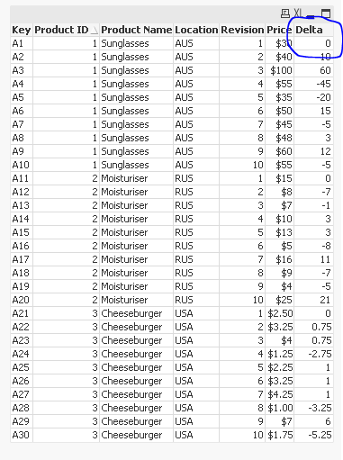
Right now delta can be positive or negative, but if you are looking for changes in either direction, you can use fabs() function which will give you the absolute value of the change
fabs(If([Product ID] = Previous([Product ID]), RangeSum(Price - Previous(Price)), 0)) as Delta
One you do this, you can use an expression like this
=Count({<[Product ID] = {1}, Delta = {'>21', '<-21'}>} [Product ID])
Right now, I hardcoded 21 and -21, but this can be driven from user input in an inputfield using a variable.
=Count({<[Product ID] = {1}, Delta = {'>$(=vDelta)', '<-$(=vDelta)'}>} [Product ID])

- Mark as New
- Bookmark
- Subscribe
- Mute
- Subscribe to RSS Feed
- Permalink
- Report Inappropriate Content
This can be handled with a little manipulation in the script
Table:
LOAD * INLINE [
Key, Product ID, Product Name, Location, Revision, Price
A1, 1, Sunglasses, AUS, 1, $30
A2, 1, Sunglasses, AUS, 2, $40
A3, 1, Sunglasses, AUS, 3, $100
A4, 1, Sunglasses, AUS, 4, $55
A5, 1, Sunglasses, AUS, 5, $35
A6, 1, Sunglasses, AUS, 6, $50
A7, 1, Sunglasses, AUS, 7, $45
A8, 1, Sunglasses, AUS, 8, $48
A9, 1, Sunglasses, AUS, 9, $60
A10, 1, Sunglasses, AUS, 10, $55
A11, 2, Moisturiser, RUS, 1, $15
A12, 2, Moisturiser, RUS, 2, $8
A13, 2, Moisturiser, RUS, 3, $7
A14, 2, Moisturiser, RUS, 4, $10
A15, 2, Moisturiser, RUS, 5, $13
A16, 2, Moisturiser, RUS, 6, $5
A17, 2, Moisturiser, RUS, 7, $16
A18, 2, Moisturiser, RUS, 8, $9
A19, 2, Moisturiser, RUS, 9, $4
A20, 2, Moisturiser, RUS, 10, $25
A21, 3, Cheeseburger, USA, 1, $2.50
A22, 3, Cheeseburger, USA, 2, $3.25
A23, 3, Cheeseburger, USA, 3, $4.00
A24, 3, Cheeseburger, USA, 4, $1.25
A25, 3, Cheeseburger, USA, 5, $2.25
A26, 3, Cheeseburger, USA, 6, $3.25
A27, 3, Cheeseburger, USA, 7, $4.25
A28, 3, Cheeseburger, USA, 8, $1.00
A29, 3, Cheeseburger, USA, 9, $7.00
A30, 3, Cheeseburger, USA, 10, $1.75
];
FinalTable:
LOAD *,
If([Product ID] = Previous([Product ID]), RangeSum(Price - Previous(Price)), 0) as Delta
Resident Table
Order By [Product ID], Revision;
DROP Table Table;
I am creating a new column called Delta where I am looking at change in the price between Revisions.
Right now delta can be positive or negative, but if you are looking for changes in either direction, you can use fabs() function which will give you the absolute value of the change
fabs(If([Product ID] = Previous([Product ID]), RangeSum(Price - Previous(Price)), 0)) as Delta
One you do this, you can use an expression like this
=Count({<[Product ID] = {1}, Delta = {'>21', '<-21'}>} [Product ID])
Right now, I hardcoded 21 and -21, but this can be driven from user input in an inputfield using a variable.
=Count({<[Product ID] = {1}, Delta = {'>$(=vDelta)', '<-$(=vDelta)'}>} [Product ID])
- Mark as New
- Bookmark
- Subscribe
- Mute
- Subscribe to RSS Feed
- Permalink
- Report Inappropriate Content
Thanks for that Sunny!
I'll have a crack at it and let you know how I go.
CT