Unlock a world of possibilities! Login now and discover the exclusive benefits awaiting you.
- Qlik Community
- :
- All Forums
- :
- QlikView App Dev
- :
- Re: Field names as column headers
- Subscribe to RSS Feed
- Mark Topic as New
- Mark Topic as Read
- Float this Topic for Current User
- Bookmark
- Subscribe
- Mute
- Printer Friendly Page
- Mark as New
- Bookmark
- Subscribe
- Mute
- Subscribe to RSS Feed
- Permalink
- Report Inappropriate Content
Field names as column headers
All,
I am wondering if it's possible to take a data set and format it like I could in a pivot table in excel. With this data set in excel, it's very easy to put location as my Row Label, Revenue Type as my Column Header, and Revenues as my sum. Why can't I seem to do this in Qlikview?
- Tags:
- new_to_qlikview
Accepted Solutions
- Mark as New
- Bookmark
- Subscribe
- Mute
- Subscribe to RSS Feed
- Permalink
- Report Inappropriate Content
Hi,
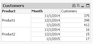
with "Revenue Type as Column Header" you mean the field values (not the field names like your thread title suggests), right?
If this is the case, then you're describing a classical pivot table.
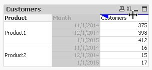
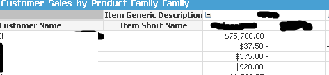
After creating one in QlikView, just drag one dimension to the top as column header:
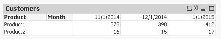
the result should look like:
hope this helps
regards
Marco
- Mark as New
- Bookmark
- Subscribe
- Mute
- Subscribe to RSS Feed
- Permalink
- Report Inappropriate Content
I'm not sure if I get what you're asking, but you can add labels for expressions, and therefore set the Field name to every expression (that'll be the column header).
Nevermind, after seeing the answer below I understood that you're looking for the field values to be the column headers. Yeah what Marco Wedel below me said is correct.
- Mark as New
- Bookmark
- Subscribe
- Mute
- Subscribe to RSS Feed
- Permalink
- Report Inappropriate Content
Hi,
with "Revenue Type as Column Header" you mean the field values (not the field names like your thread title suggests), right?
If this is the case, then you're describing a classical pivot table.
After creating one in QlikView, just drag one dimension to the top as column header:
the result should look like:
hope this helps
regards
Marco
- Mark as New
- Bookmark
- Subscribe
- Mute
- Subscribe to RSS Feed
- Permalink
- Report Inappropriate Content
That does it. Thanks Guys!
- Mark as New
- Bookmark
- Subscribe
- Mute
- Subscribe to RSS Feed
- Permalink
- Report Inappropriate Content
You're welcome
regards
Marco
- Mark as New
- Bookmark
- Subscribe
- Mute
- Subscribe to RSS Feed
- Permalink
- Report Inappropriate Content
Can the columns be moved? To use your example above, could you drag December in front of November?
- Mark as New
- Bookmark
- Subscribe
- Mute
- Subscribe to RSS Feed
- Permalink
- Report Inappropriate Content
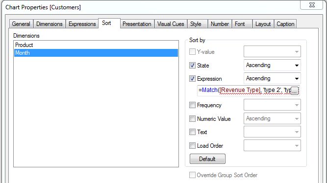
not by dragging, you would have to define a special sort order, e.g. an expression to sort by.
- Mark as New
- Bookmark
- Subscribe
- Mute
- Subscribe to RSS Feed
- Permalink
- Report Inappropriate Content
one example:
=Match([Revenue Type], 'type 2', 'type 3', 'type 1')
would sort the Revenue Type columns in the defined order: 'type 2', 'type 3', 'type 1'
hope this helps
regards
Marco
- Mark as New
- Bookmark
- Subscribe
- Mute
- Subscribe to RSS Feed
- Permalink
- Report Inappropriate Content
Sorry to keep pestering you - but any idea why I am not seeing any subtotals? 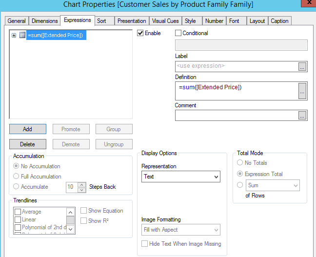
- Mark as New
- Bookmark
- Subscribe
- Mute
- Subscribe to RSS Feed
- Permalink
- Report Inappropriate Content
No, not at the first glance.