Unlock a world of possibilities! Login now and discover the exclusive benefits awaiting you.
- Qlik Community
- :
- All Forums
- :
- QlikView App Dev
- :
- How to get Score in Text Object overall month wise...
- Subscribe to RSS Feed
- Mark Topic as New
- Mark Topic as Read
- Float this Topic for Current User
- Bookmark
- Subscribe
- Mute
- Printer Friendly Page
- Mark as New
- Bookmark
- Subscribe
- Mute
- Subscribe to RSS Feed
- Permalink
- Report Inappropriate Content
How to get Score in Text Object overall month wise Score
Hi,
I need to show the top 3 store ID based on the score over the month.
This is i can able to see in the 'straight table' but i could not able show in the 'text object'.
My score expression is (Sum(A+B+C)/Sales)*1000 , Here I need to categorize in to 3 groups.
1) Score which is <= 20 , I need to show the store name whose score start from "0". and their sales.
2) Score >20 and <=50, Here i need to show top 3 score store names and their score as well
3) Score >50, Here also i need to show top 3 score store names and their score as well.
| Date | Store Name | A | B | C | Sales | Score |
|---|---|---|---|---|---|---|
| 01-01-2018 | ABC | 25 | 10 | 5 | 40 | 3.4568 |
| 02-01-2018 | DEF | 2 | 9 | 10 | 21 | 3.4863 |
| 03-01-2018 | LMN | 62 | 56 | 5 | 123 | 5.896 |
| 04-01-2018 | PQR | 20 | 5 | 3 | 28 | 45.5689 |
| 01-02-2018 | ABC | 5 | 9 | 12 | 26 | 6.852 |
| 02-02-2018 | DEF | 35 | 16 | 8 | 59 | 64.852 |
| 03-02-2018 | LMN | 5 | 9 | 15 | 29 | 2.6541 |
| 04-02-2018 | PQR | 5 | 2 | 3 | 10 | 3.2598 |
| 01-03-2018 | ABC | 6 | 140 | 85 | 231 | 80.258 |
| 02-03-2018 | LMN | 52 | 46 | 75 | 173 | 77.264 |
| 03-03-2018 | DEF | 49 | 52 | 25 | 126 | 4.258 |
| 04-03-2018 | PQR | 2 | 2 | 3 | 7 | 0.451 |
More Information Please refer below Excel.
Thanks,
Ravi.
- « Previous Replies
-
- 1
- 2
- Next Replies »
- Mark as New
- Bookmark
- Subscribe
- Mute
- Subscribe to RSS Feed
- Permalink
- Report Inappropriate Content
based on your excel sheet try something like this? And not sure about your 1st point you mentions saying you want values 0. Could you elaborate on that please like what values you are expecting to see for your 1st requirement. For now i am showing top 3 values for all the 3 conditions. Try below:
SampleFile:
LOAD
Month(Floor(Num#(Date#(Date, 'M/DD/YYYY')))) AS MonthName,
Date AS StoreDate,
[STORE Name] AS StoreName,
A,
B,
C,
sales,
score
FROM
[..\SampleData1.xls]
(biff, embedded labels, table is Sheet1$);
LEFT JOIN(SampleFile)
LOAD *,
IF(ScoreValue <= 20, 'Grp1',
IF(ScoreValue > 20 AND ScoreValue <=50, 'Grp2',
IF(ScoreValue > 50, 'Grp3'))) AS GroupFlg;
LOAD StoreDate,
sales,
(Sum(A+B+C)/sales)*1000 AS ScoreValue
Resident SampleFile
Group By StoreDate,A,B,C,sales;
Using straight table added:
Dim: Storename, sales, GroupFlg
Expr: = Num(IF(Aggr(Rank(Sum(ScoreValue)), GroupFlg,StoreName) <=3, ScoreValue), '#,##0.000')
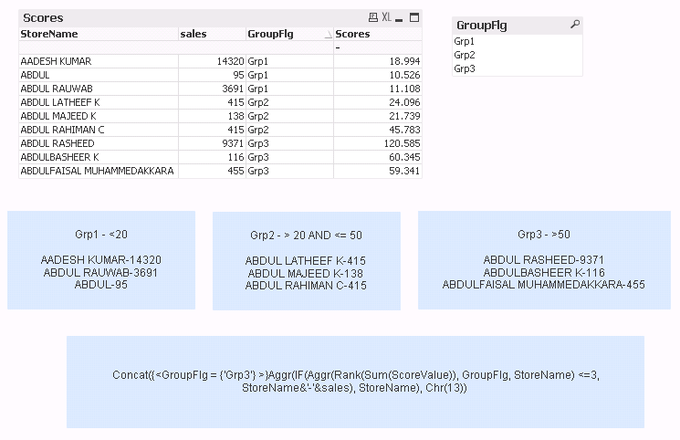
In the image above the below 3 text boxes show top 3 scores for different groups.
let us know if this is not what you are looking for. We can dig through. The big text box in the bottom shows what expr i have used in those 3 textobjects to get top 3.
- Mark as New
- Bookmark
- Subscribe
- Mute
- Subscribe to RSS Feed
- Permalink
- Report Inappropriate Content
Hi Vishwarath,
Thanks for your valuable support.
please find attached QVW file which we are implemented as per your suggestion,
Still I am struggling to show the proper result, please find attachment.
- Mark as New
- Bookmark
- Subscribe
- Mute
- Subscribe to RSS Feed
- Permalink
- Report Inappropriate Content
Did the requirement changed? The file i am looking at does not have top 3 scores. Can you explain a little more of why SARDARA has to come in Green flag.
I believe the data your produced in your excel does not work here as you have to sum([Km Traveled]) and sum of HA Count and other fields to be included. Can you share your Safety SND Report.xlsx file so that i can run and change the expressions accordingly.
Mean while you can try like below:
LEFT JOIN(SampleFile)
LOAD *,
IF(Safetyscore <= 20, 'Green',
IF(Safetyscore > 20 AND Safetyscore <=50, 'Yellow',
IF(Safetyscore > 50, 'Red'))) AS GroupFlg;
LOAD //StoreDate,
[Vehicle Number],
//TravelledDate,
//[OVSD Count],
//[HA Count],
//[HB Count],
//[CD Count],
// sales,
(RangeSum(sum([OVSD Count]), Sum([HA Count]), Sum([HB Count]), Sum([CD Count]))/Sum([Kms Travelled]))) * 1000 as Safetyscore
Resident SampleFile
Group By [Vehicle Number];
- Mark as New
- Bookmark
- Subscribe
- Mute
- Subscribe to RSS Feed
- Permalink
- Report Inappropriate Content
Hi Viswarath,
Thanks for your reply.Tried with above script.
Here i selected carrierCode "916002585"
so that in Green Category the highest kms travelled 4991 "SARDARA SINGH". If i select month name should change the based on the highest kms travelled.
In green we need consider kms travelled. and Yellow & Red we should consider the Highest score.
Please find the attached
- Mark as New
- Bookmark
- Subscribe
- Mute
- Subscribe to RSS Feed
- Permalink
- Report Inappropriate Content
OK not sure what is your expected output is. Can you elaborate. So where and what you want to see in your sheet when you select CarrierCode can you tell me the output you want to see?
- Mark as New
- Bookmark
- Subscribe
- Mute
- Subscribe to RSS Feed
- Permalink
- Report Inappropriate Content
Thanks Vishwarath,
Sure,
> First thing I want to show in text object the No. of Green Kms travelled drivers , Yellow and red kms travelled Drivers.
> Along with this information as i discussed, the below information also i should provide in the Text objects.
> Top 5 Green Driver Names based KMS travelled and their kms, Top 5 Yellow drivers based on their score and top 5 Red drivers based in their score.
(If Score is high that Driver is comes in 1st place, Next high score driver name is comes in 2nd place etc)
These score will be aggregate over the month.
Score =(sum([CD Count]+[HA Count]+[OVSD Count]+[HB Count])/sum([Kms Travelled])) *1000
1) Green -> Score<=20
2) Yellow -> Score 20 -50
3) Red -> Score above 50
.
Please let me know if any other information.
- Mark as New
- Bookmark
- Subscribe
- Mute
- Subscribe to RSS Feed
- Permalink
- Report Inappropriate Content
Will look into it tomorrow.
- Mark as New
- Bookmark
- Subscribe
- Mute
- Subscribe to RSS Feed
- Permalink
- Report Inappropriate Content
Hi Vishwarath,
Thanks for your great support!!
I tried a lot for this task, but still its not resolved. Is there any chances from your end?
can you please help me on this?
Thanks,
Ravi.
- Mark as New
- Bookmark
- Subscribe
- Mute
- Subscribe to RSS Feed
- Permalink
- Report Inappropriate Content
Sorry Ravi for late response. I was so caught up with my child could not able to look into this. I will look into it today and get back. Can i know what timezone you work in?
- « Previous Replies
-
- 1
- 2
- Next Replies »