Measuring variation between columns

[Anonymous]

Hi

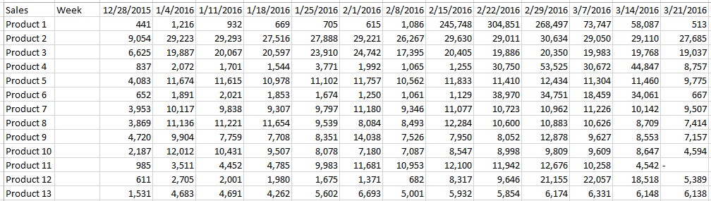
I have this Pivot Table, with 2 dimensions. One dimension is Product Id, and the 2nd one is Week, that I move it as an horizontal dimension. An the metric is Sales. So here I can quickly check sales per Product Week over Week and for example find out that Product 1 last week sales drooped a lot.

My questions are

1-How can I make an expression to measure variation over previous column?, instead of showing the sales value of the week.

2-How can I sort 1st dimension. Product Id, considering total sales Desc and not only last column.

Thanks in advance for you help!

[Gysbert_Wassenaar · Accepted solution]

1. Use something like sum(Sales)/before(sum(Sales))

2. Try sorting by expression. Perhaps =sum(Total <[Product Id]>Sales)