Recipe for a Pareto Analysis

[hic]

“Which products contribute to the first 80% of our turnover?”

[hic]

This type of question is common in all types of business intelligence. I say “type of question” since it appears in many different forms: Sometimes it concerns products, but it can just as well concern customers, suppliers or sales people. It can really be any dimension. Further, here the question was about turnover, but it can just as well be number of support cases, or number of defect deliveries, etc. It can in principle be any additive measure.

It is called Pareto analysis. Sometimes also known as 80/20 analysis or ABC analysis.

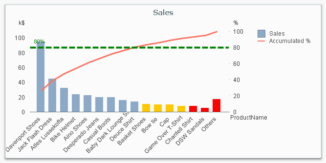
The logic is that you first sort the products according to size, then accumulate the numbers, and finally calculate the accumulated measure as a percentage of the total. The products contributing to the first 80% are your best products; your “A” products. The next 10% are your “B” products, and the last 10% are your “C” products.

And here’s how you do it in QlikView:

1. Create a pivot table and choose your dimension and your basic measure. In my example, I use Product and Sum(Sales).
   
   
2. Sort the chart descending by using the measure Sum(Sales) as sort expression. It is not enough just to check “Sort by Y-value”.
   
   
3. Add a second expression to calculate the accumulated sales value:
        RangeSum(Above(Sum(Sales), 0, RowNo()))
   Call this expression Accumulated Sales. The Above() function will return an array of values – all above values in the chart – and the RangeSum() function will sum these numbers.
   
   
4. Create a third expression from the previous one; one that calculates the accumulated sales in percent:
        RangeSum(Above(Sum(Sales), 0, RowNo())) / Sum(total Sales)
   Format it as a percentage and call it Inclusive Percentage.
   
   
5. Create a fourth expression from the previous one; one that calculates the accumulated sales in percent, but this time excluding the current row:
         RangeSum(Above(Sum(Sales), 1, RowNo())) / Sum(total Sales)
   Format it as a percentage and call it Exclusive Percentage.
   
   
6. Create a fifth expression for the ABC classification:
         If([Exclusive Percentage] <= 0.8, 'A', If([Exclusive Percentage] <= 0.9, 'B', 'C'))
   Call this expression Pareto Class. The reason why the Exclusive Percentage is used, is that the classification should be determined by the lower bound of a product’s segment, not the upper.
   
   
7. Create a conditional background color, e.g.
         If([Pareto Class] = 'C', LightRed(), If([Pareto Class] = 'B', Yellow()))

You should now have a table similar to the following. In it you can clearly see the classification of different products.

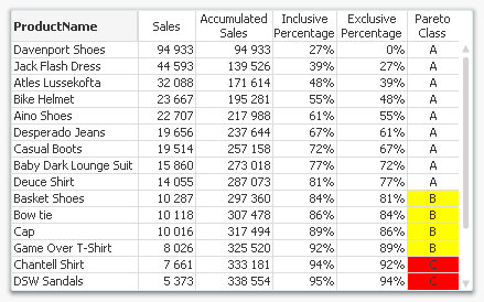
In this table, there are five different expressions that you can use for Pareto analysis. The graph in the beginning of this post uses Sales and Inclusive Percentage for the bars and the line, respectively; and Pareto Class for the coloring of the bars.

Further, you may want to combine the Pareto Class and the Exclusive Percentage into one expression:

     Pareto Class =
         If(RangeSum(Above(Sum(Sales),1,RowNo())) / Sum(total Sales) <= 0.8, 'A',
         If(RangeSum(Above(Sum(Sales),1,RowNo())) / Sum(total Sales) <= 0.9, 'B', 'C'))

Good luck in creating your Pareto chart.

HIC

Further reading related to this topic:

Recipe for an ABC Analysis

Recipe for a Pareto Analysis – Revisited

[carolin01]

Ok, this worked fine so far. My problem is now the following values for my smaller customers:

I think there is again a mistake in my formula:

RangeSum(Above($(vCalcTotalYear1), 0, RowNo()))) /( $(vCalcTotalYear1))/100

Or should I just try to format the second axis for the combo chart? In this case I´m not sure how to do this.

My other formulas look like this:

Sales:

$(=vCalcTotalYear1)

Accumulted Sales

RangeSum(Above($(vCalcTotalYear1), 0, RowNo()))

Inclusive Percentage

RangeSum(Above($(vCalcTotalYear1), 0, RowNo()))) /( $(vCalcTotalYear1))/100

Exclusive Percentage

RangeSum(Above($(vCalcTotalYear1), 1, RowNo()))) /( $(vCalcTotalYear1))/100

Pareto Class

If([Exclusive Percentage] <= 0.8, 'A', If([Exclusive Percentage] <= 0.9, 'B', 'C'))

If I format the table as pivot then accumulated Sales is correct. If I format it as Straight table then it´s incorrent.  Straight Table:

[hic]

You cannot have the same variable in the numerator as in the denominator.

Numerator should have Sum(Sales)

Denominator should have Sum(total Sales)

Further, you do not need to divide by 100. Just format it as percentage and it will automatically display it correctly.

HIC

[#5]

Hi Henric,

Thanks for such a detailed solution. Everything works fine for me except the reference line. Firstly I want to understand why we are using secondary Y for reference line. Reference line comes up nicely using Primary Y but does not show up using the secondary Y . Please help.

Thanks

Abhishek

[hic]

It depends what you have as primary and secondary Y. In my example, the primary Y is Sum(Sales) which is typically 30000$, and the secondary is the relative percentage, i.e. a number between 0 and 1.

Primary and secondary are defined through the Left and Right Axis on the Axes tab.

HIC

[#7]

I missed the right hand axis part for second dimension. Now I think I got it wright. Thanks for the quick help Henric. The reference line is also working for secondary Y now.

I have another question. Can we show the products in x- axis as percentage?

I tried with a calculated dimension like   "RowNo()/Count(Products)" .

I want to achieve this so that we can show clearly "First 20% products are contributing to 80% of the Sales"

[hic]

You could use

     Count(distinct Product)/Count(distinct total Product)

as expression to calculate such a percentage.

But if you want a calculated dimension, I am not so sure what it would be...

HIC

[dmohanty]

Hi Henric,

Thanks for this excellent post.

Also, I was showing the Accumulated Sales % Now I want to show two Referal Lines (black dotted line): one for Top 5 and other for Top 10. How can I show it dynamically?

Here is the image below:

[Anonymous]

I find also useful add an expression RowNo() with Text on Axis as Display Option

so you can easily know how many products make the 80% of revenue

[hic]

I would create a reference line for the top 5 using

Sum(Aggr(If(Rank(Sum (Sales))<=5,Sum (Sales)),ProductName)) / Sum (Sales)

HIC

[dmohanty]

Great Henric. It really helped in acheiving my requirement.

Learnt a new thing from this as well. Thank you very much for this!