Native statistical functions are used very little by Qlik developers as far as I know. Those with data science background stick to standard tools like R and Phyton. Using these along with Qlik was made easier by server-side extensions and previously impossible use cases are now simple and straightforward.
You can learn more about SSE here: https://github.com/qlik-oss/server-side-extension
Nevertheless, it would be a shame to completely disregard native Qlik functions. With little effort (and without SSE link to external statistical engine) they can help us to enrich loaded data and help to find unexpected insights.
For example, one use case, that I would like to examine here, is to segment customers with a help of linear regression. The simplest approach is to focus on sales by customers in time.
Using linear regression in a chart expression can give us following information.
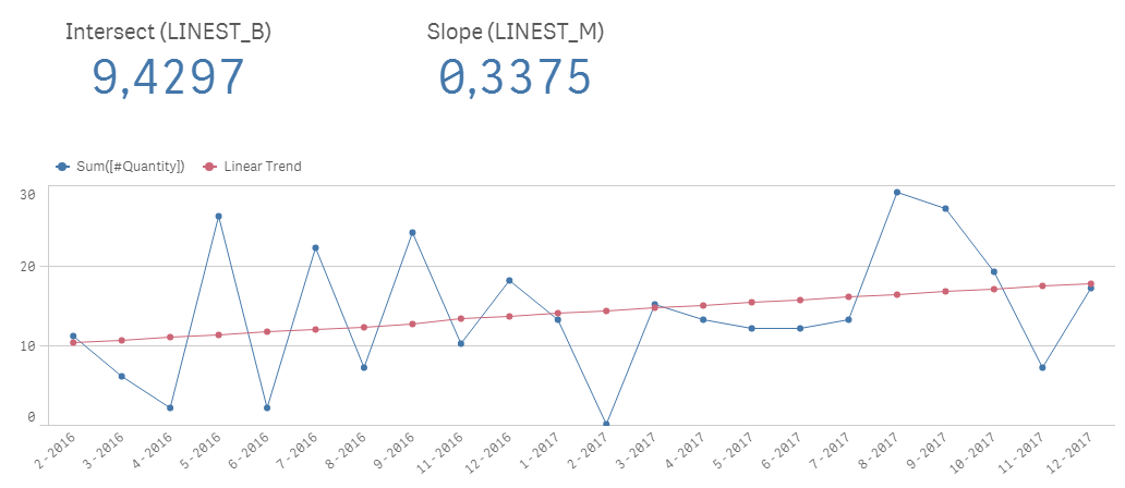
The expression for the regression line is the following:

LINEST_B function calculates the intersect – initial value when the independent variable is zero
LINEST_M function calculates the slope of the regression line
(field “MonthSeq“ is just a sequential number for months starting from 1)
Having a dynamic expression for any combination of selected dimensions is an awesome way to familiarize oneself with data and underlying linear trends in them.
When our focus is on data discovery, it’s often better to pre-calculate regression in the script. For example, we could seek only those customers whose general trend is negative and for that we need some handle (field) for selection.
Obviously, first we must have some transactional data prepared. I created a testing script for this exercise, which will create a dataset (it uses random numbers so after each reaload the results will change).
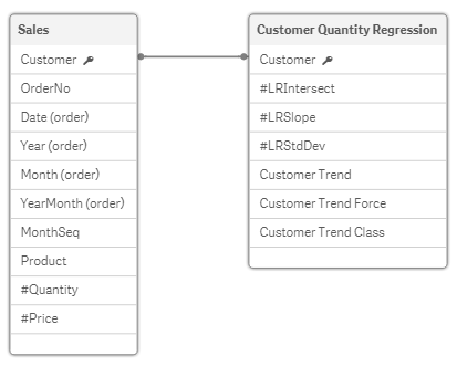
Our goal is to associate a new table with this data, which will store the regression results on defined level. For the sake of simplicity, we will calculate on a customer level only.
Next, we choose two numerical fields which will be used in linear regression algorithm (Qlik’s LR functions support only two fields, for multi-variate regression one must use SSE to a statistical engine).
Since we want to calculate a linear trendline for sales quantity, one value will represent the order position of a particular month of the year and a second value will be a sum of quantity sold in that month. Therefore, we create a resident aggregate table which will sum the quantity by customer and month sequence number.
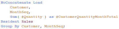
The month sequence number is calculated in the script using autonumber function on top of month-year ID.

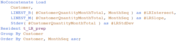
Now we are ready to use regression functions. We’ll make calculations in another resident table. The resulting dataset will store regression coefficients, intersect and slope, and I usually add also a standard deviation, which gives a good information about how spread out the underlying values are.
Numbers are nice, but I like to also make some basic categorizations for quicker filtering . Thus, we will add trend orientation (positive or negative), trend force (significant or negligible) and trend classes. This can be done by preceding load on top of the last resident table.
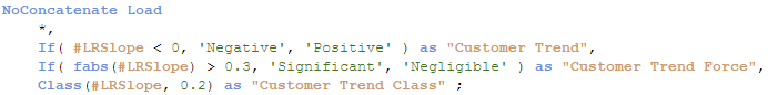
We used suitable constants for the trend force and class in this example, but I recommend to use quartiles in a real-world scenario.
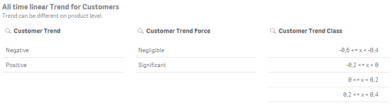
Resulting data model includes fields that will allow us e.g. to quickly filter customers with significant negative trend.
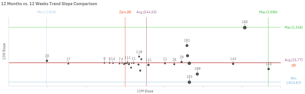
Real-world data allow us to go much further. First, there can be multiple levels of calculation, like country, site, customer, item, operation, service, etc. and even their combinations. Then, regression can be calculated in multiple time frames – 12 months, 12 weeks, 30 days... And, there usually is a great number of different measures, so the regression can be calculated not only against time but also in between them.
The most fun (and insightful) is then to cross-analyze all these regressions against each other using Qlik’s associative experience.
Linear regression is not suitable for predictions but I found that it can serve as a very effective navigator for business users who do not have statistical background and have larger detailed datasets.
Check the attached file to see expressions as well as described script. I’m looking forward to hearing any comments and suggestions.
Radovan
PS: If you'd like to use power or polynomial trendline, check Calculating trend lines, values and formulas on charts and tables in Qlik Sense by richbyard.
