Unlock a world of possibilities! Login now and discover the exclusive benefits awaiting you.
- Qlik Community
- :
- All Forums
- :
- QlikView App Dev
- :
- Excluding values from table
- Subscribe to RSS Feed
- Mark Topic as New
- Mark Topic as Read
- Float this Topic for Current User
- Bookmark
- Subscribe
- Mute
- Printer Friendly Page
- Mark as New
- Bookmark
- Subscribe
- Mute
- Subscribe to RSS Feed
- Permalink
- Report Inappropriate Content
Excluding values from table
Hello!
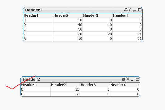
In straight I need to show only those value which have "zero" in cells. For example,
| Header 1 | Header 2 | Header 3 | Header 4 |
|---|---|---|---|
| A | 10 | 0 | 12 |
| B | 20 | 0 | 0 |
| C | 30 | 20 | 11 |
| D | 40 | 10 | 0 |
| E | 50 | 0 | 0 |
As a result of formula, the table should transform to the following:
| Header 1 | Header 2 | Header 3 | Header 4 |
|---|---|---|---|
| B | 20 | 0 | 0 |
| E | 50 | 0 | 0 |
Kind regards,
Ruslan
- Tags:
- formula
- table filter
- « Previous Replies
-
- 1
- 2
- Next Replies »
Accepted Solutions
- Mark as New
- Bookmark
- Subscribe
- Mute
- Subscribe to RSS Feed
- Permalink
- Report Inappropriate Content
Also, suppress the NULLS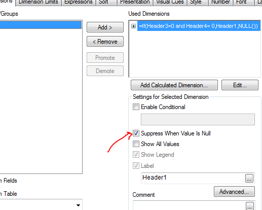
- Mark as New
- Bookmark
- Subscribe
- Mute
- Subscribe to RSS Feed
- Permalink
- Report Inappropriate Content
From where you want this back end or in front end?
- Mark as New
- Bookmark
- Subscribe
- Mute
- Subscribe to RSS Feed
- Permalink
- Report Inappropriate Content
Do it at script level, create a flag to see where we have all zeroes and then create a calculated dimension using that flag.
Refer attached.
- Mark as New
- Bookmark
- Subscribe
- Mute
- Subscribe to RSS Feed
- Permalink
- Report Inappropriate Content
- Mark as New
- Bookmark
- Subscribe
- Mute
- Subscribe to RSS Feed
- Permalink
- Report Inappropriate Content
Where I should insert the code in script because flagging seems doesn't work.
Directory;
LOAD Index,
[Company name],
Header 3,
FROM [0_ISS\Processed\ProcPopulation 31.12.2016.xlsx] (ooxml, embedded labels, table is Sheet1);
Directory;
LOAD Index,
Header 4,
FROM [0_ISS\Processed\ProcPopulation 01.01.2017-20.05.2017.xlsx]
(ooxml, embedded labels, table is Sheet1);
LOAD
If([CR, Оплачено]=0 and Оплачено=0,0,1) as Flag;
- Mark as New
- Bookmark
- Subscribe
- Mute
- Subscribe to RSS Feed
- Permalink
- Report Inappropriate Content
Directory;
Load * , If(Header3=0 ,0,1) as Flag
LOAD Index,
[Company name],
Header 3,
FROM [0_ISS\Processed\ProcPopulation 31.12.2016.xlsx] (ooxml, embedded labels, table is Sheet1);
Directory;
Load * , If(Header4=0,0,1) as Flag
LOAD Index,
Header 4,
FROM [0_ISS\Processed\ProcPopulation 01.01.2017-20.05.2017.xlsx]
(ooxml, embedded labels, table is Sheet1);
- Mark as New
- Bookmark
- Subscribe
- Mute
- Subscribe to RSS Feed
- Permalink
- Report Inappropriate Content
You can also do it at the front end-
Just use a calculated dimension-
=If(Header3=0 and Header4= 0,Header1,NULL())
- Mark as New
- Bookmark
- Subscribe
- Mute
- Subscribe to RSS Feed
- Permalink
- Report Inappropriate Content
Refer this. Without flagging at Front end.
- Mark as New
- Bookmark
- Subscribe
- Mute
- Subscribe to RSS Feed
- Permalink
- Report Inappropriate Content
Also, suppress the NULLS
- Mark as New
- Bookmark
- Subscribe
- Mute
- Subscribe to RSS Feed
- Permalink
- Report Inappropriate Content
Are you making a new table after these two loads for Header3 & Header4 as zero?
- « Previous Replies
-
- 1
- 2
- Next Replies »