Unlock a world of possibilities! Login now and discover the exclusive benefits awaiting you.
- Qlik Community
- :
- All Forums
- :
- QlikView App Dev
- :
- Re: I am trying to compare different values in a s...
- Subscribe to RSS Feed
- Mark Topic as New
- Mark Topic as Read
- Float this Topic for Current User
- Bookmark
- Subscribe
- Mute
- Printer Friendly Page
- Mark as New
- Bookmark
- Subscribe
- Mute
- Subscribe to RSS Feed
- Permalink
- Report Inappropriate Content
I am trying to compare different values in a single straight chart
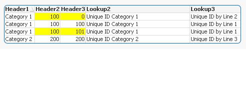
I am trying to compare different pieces of data within a single straight chart. In the chart below, I want to use a color highlight for any different values in Header 2 and Header 3. How would I write this if I wanted to say if the value in Lookup2 matches, then highlight the cells in Header 2 and Header 3 if the values are different? Thank you very much for your help.
| Header 1 | Header 2 | Header 3 | LOOKUP2 | Lookup3 |
| Category 1 | 100 | 100 | Unique ID Category 1 | Unique ID by Line 1 |
| Category 1 | 100 | 0 | Unique ID Category 1 | Unique ID by Line 2 |
| Category 2 | 200 | 200 | Unique ID Category 2 | Unique ID by Line 3 |
| Category 2 | 300 | 300 | Unique ID Category 2 | Unique ID by Line 4 |
| Category 3 | 50 | 50 | Unique ID Category 3 | Unique ID by Line 5 |
| Category 3 | 60 | 60 | Unique ID Category 3 | Unique ID by Line 6 |
| Category 4 | 100 | 100 | Unique ID Category 4 | Unique ID by Line 7 |
| Category 4 | 100 | 100 | Unique ID Category 4 | Unique ID by Line 8 |
| Category 5 | 300 | 300 | Unique ID Category 5 | Unique ID by Line 9 |
| Category 5 | 400 | 400 | Unique ID Category 5 | Unique ID by Line 10 |
- Mark as New
- Bookmark
- Subscribe
- Mute
- Subscribe to RSS Feed
- Permalink
- Report Inappropriate Content
I am not getting you, Can you elaborate more, Please?
- Mark as New
- Bookmark
- Subscribe
- Mute
- Subscribe to RSS Feed
- Permalink
- Report Inappropriate Content
What I am trying to do is for all rows where the Unique ID Category match, compare the values under the columns Header 2 and Header 3. Where they are not equal, I want to either have them show up as a different color, or possibly have a column next to them saying "do not match". So for the first two lines, they both have Unique ID category1. The two values under Header 2 match so I would leave them alone. The two values under Header 3 do not match, so I would want to highlight them differently.
Does this make it clearer? If so, do you have any ideas?
- Mark as New
- Bookmark
- Subscribe
- Mute
- Subscribe to RSS Feed
- Permalink
- Report Inappropriate Content
It is still confusing.. But can you take a look at the attached and see if that is what you want...
- Mark as New
- Bookmark
- Subscribe
- Mute
- Subscribe to RSS Feed
- Permalink
- Report Inappropriate Content
That is almost what I was intending. You are comparing items from Header 2 to Header 3. What I am trying to compare is lines Vertically. So for the first two lines under the Column Header 3, the values are 100 and 0 and they both have the same value under lookup 2. It's the 100 to 0 that we want to compare and highlight as different.
- Mark as New
- Bookmark
- Subscribe
- Mute
- Subscribe to RSS Feed
- Permalink
- Report Inappropriate Content
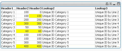
See if the attached is what you are expecting:
- Mark as New
- Bookmark
- Subscribe
- Mute
- Subscribe to RSS Feed
- Permalink
- Report Inappropriate Content
Or if you want to color both above and below, then you can try
Used Thirumala's sample and made slight modifications
- Mark as New
- Bookmark
- Subscribe
- Mute
- Subscribe to RSS Feed
- Permalink
- Report Inappropriate Content
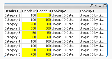
This is getting closer but when I applied the solution to my document, I noticed a problem. Lets us the column Header 2 as an example. The third and fourth row have the same value in the column Lookup2 so we want to compare them together and highlight them if the numbers in Header 2 are different. In this case, the numbers are 200 and 300 so they are being highlighted. However, if the first two rows under Header 2 match row 3, it won't be highlighted even though it does not match row 4. I need a way to have them only compare against each other when they have the same value in Lookup 2. Any ideas here?