Unlock a world of possibilities! Login now and discover the exclusive benefits awaiting you.
- Qlik Community
- :
- All Forums
- :
- QlikView App Dev
- :
- Re: Display zero values but do NOT rank them
- Subscribe to RSS Feed
- Mark Topic as New
- Mark Topic as Read
- Float this Topic for Current User
- Bookmark
- Subscribe
- Mute
- Printer Friendly Page
- Mark as New
- Bookmark
- Subscribe
- Mute
- Subscribe to RSS Feed
- Permalink
- Report Inappropriate Content
Display zero values but do NOT rank them
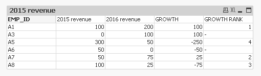
Hi, I have a requirement to display all values in pivot chart but rank ONLY non-zero values. Below is the base data with expected Rank in last column: (If 2015 or 2016 revenue is zero, do NOT Rank them)
Expected Result:
| EMP_ID | 2015 REVENUE | 2016 REVENUE | GROWTH (2016-2015) | GROWTH RANK |
| A1 | 100 | 200 | 100 | 1 |
| A3 | 0 | 100 | 100 | |
| A5 | 300 | 50 | -250 | 4 |
| A6 | 50 | 0 | -50 | |
| A7 | 50 | 75 | 25 | 2 |
| A8 | 100 | 25 | -75 | 3 |
If I give ROWTH RANK = IF ([2015 REVENUE] <> 0 AND [2016 REVENUE] <> 0, Rank([GROWTH],0,1), ' ' ) I am getting below result which is not I need.
| EMP_ID | 2015 REVENUE | 2016 REVENUE | GROWTH (2016-2015) | GROWTH RANK |
| A1 | 100 | 200 | 100 | 1 |
| A3 | 0 | 100 | 100 | |
| A5 | 300 | 50 | -250 | 6 |
| A6 | 50 | 0 | -50 | |
| A7 | 50 | 75 | 25 | 3 |
| A8 | 100 | 25 | -75 | 5 |
- Tags:
- rank ignoring zero
- Mark as New
- Bookmark
- Subscribe
- Mute
- Subscribe to RSS Feed
- Permalink
- Report Inappropriate Content
Try this:
Rank(If([2015 REVENUE] <> 0 and [2016 REVENUE] <> 0, [GROWTH]), 0, 1)
- Mark as New
- Bookmark
- Subscribe
- Mute
- Subscribe to RSS Feed
- Permalink
- Report Inappropriate Content
Didn't work. It gave ranks as 1,1,6,4,3,5. I am expecting 1,space,4,space,2,3
- Mark as New
- Bookmark
- Subscribe
- Mute
- Subscribe to RSS Feed
- Permalink
- Report Inappropriate Content
Would you be able to share a sample?
- Mark as New
- Bookmark
- Subscribe
- Mute
- Subscribe to RSS Feed
- Permalink
- Report Inappropriate Content
@ Sunny, Attached the test qvw for reference.
- Mark as New
- Bookmark
- Subscribe
- Mute
- Subscribe to RSS Feed
- Permalink
- Report Inappropriate Content
I think the field names were not right. You used _ in your field name which was missing
=Rank(If([2015_REVENUE] <> 0 and [2016_REVENUE] <> 0, [GROWTH]), 0, 1)
- Mark as New
- Bookmark
- Subscribe
- Mute
- Subscribe to RSS Feed
- Permalink
- Report Inappropriate Content
OR Get rid off these If condition and Use Pick / Match :
Rank(Pick(-1*(not match(RangeSum([2015_REVENUE]+[2016_REVENUE]),[2015_REVENUE],[2016_REVENUE])),[GROWTH]), 0, 1)
- Mark as New
- Bookmark
- Subscribe
- Mute
- Subscribe to RSS Feed
- Permalink
- Report Inappropriate Content
Might be better performing (not sure)... but looks way more complicated.... def. give it a shot though 