Max of columns in pivot table which are already calculated by BEFORE() function... Nesting BEFORE() and BELOW()?

[#1]

Hey all,

I have the following problem regarding a QlikView App where many values have to be calculated on the fly based on the user selection.

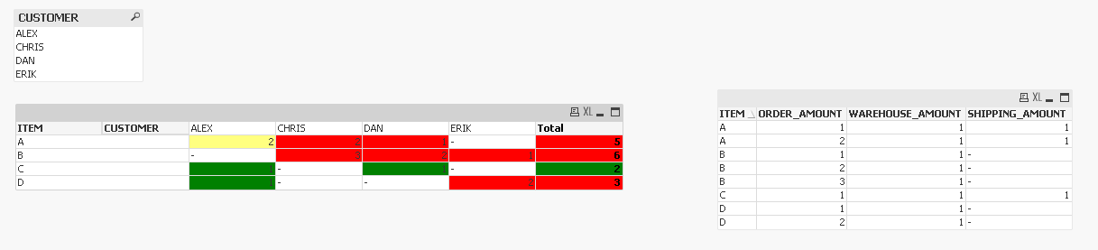
Suppose I have a shop with items A, B, C, D. Some amount is in the warehouse. Some of them are currently shipped to the warehouse.

And I have customers ordering the items.

Now I want to display a pivot table with customers and the items showing in the cells the amount they ordered.

The cells should get a background color based on whether the amount can be fully covered by the warehouse --> green, or by the items currently shipped to the warehouse --> yellow, or otherwise --> red.

The customers get sorted by their registration date and should be served according to the registration date.

i.e. first customer orders item A two times, second customer orderes item A one time. Two As are in the warehouse --> First customer gets the items from the warehouse, second customer and item A are displayed in red.

Now if the user only selects second customer, the cell is green. 

That is why I can not calculate any of the colors in the script. Everything is based on which customers the user selects. 

I managed to get that by using the BEFORE() function in the pivot table and calculate RangeSums.

See attached file.

Everything is working fine. 

What I now would like to have is an overall status for the customers:

(Every column should get an overall status)

Can the complete order be covered by warehouse etc.?

If at least one item of the customer order is red, then the customer would be displayed in red.

otherwise if at least one item is yellow, customer is yellow, otherwise green.

Any help or tips and tricks are highly appreciated. Thank you!

[sunny_talwar]

If you enable Partial Sum on the presentation tab, isn't that is already done for you?

[#3]

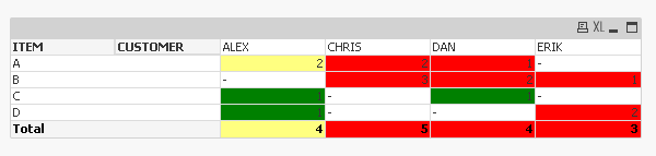
Thank you. That would do the trick if I would want the total of each item.

But I want the total of each customer.

So if I enable partial sum for the other dimension, it sums up the items per customer, but the color is not doing what i want:

Total of customer Alex should be yellow.

[sunny_talwar]

May be try this:

=If(Dimensionality() = 0,

Pick(Max(Aggr(If(sum(ORDER_AMOUNT) > 0,

If(ORDER_AMOUNT + if(Rangesum(BEFORE(TOTAL ORDER_AMOUNT,1,count(distinct CUSTOMER)))>0,Rangesum(BEFORE(TOTAL ORDER_AMOUNT,1,count(distinct CUSTOMER))), 0) <= WAREHOUSE_AMOUNT, 1,

if(ORDER_AMOUNT + if(Rangesum(BEFORE(TOTAL ORDER_AMOUNT,1,count(distinct CUSTOMER)))>0,Rangesum(BEFORE(TOTAL ORDER_AMOUNT,1,count(distinct CUSTOMER))), 0) <= WAREHOUSE_AMOUNT + SHIPPING_AMOUNT, 2,

3)),

4), CUSTOMER, ITEM)), RGB(0,128,0), RGB(255,255,128), RGB(255,0,0), RGB(255,255,255)),

If(sum(ORDER_AMOUNT) > 0,

If(ORDER_AMOUNT + if(Rangesum(BEFORE(TOTAL ORDER_AMOUNT,1,count(distinct CUSTOMER)))>0,Rangesum(BEFORE(TOTAL ORDER_AMOUNT,1,count(distinct CUSTOMER))), 0) <= WAREHOUSE_AMOUNT, RGB(0,128,0),

if(ORDER_AMOUNT + if(Rangesum(BEFORE(TOTAL ORDER_AMOUNT,1,count(distinct CUSTOMER)))>0,Rangesum(BEFORE(TOTAL ORDER_AMOUNT,1,count(distinct CUSTOMER))), 0) <= WAREHOUSE_AMOUNT + SHIPPING_AMOUNT, RGB(255,255,128),

RGB(255,0,0))),

RGB(255,255,255)))

[#5]

Great! Thank you so much.

It is working on the first sight, but if I expand my example by customer Steve who wants to order item A, B and C each one time,

things get confused.

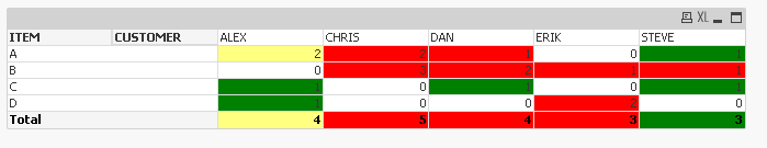
Item A should be red for Steve, as he is the last customer to be served and Chris and Dan don't get item A neither.

Item C should also be red for Steve as there is only one piece of C in the warehouse (Alex gets that) and one piece in the shipping process (Dan gets that) and therefore the cell "Dan - Item C" should be yellow.

Overall Steve should be red. 

So I think I understand your expression and it is really well done, but unfortunately it is not doing what I would expect.

[sunny_talwar]

This was not an issue with your existing expression? I did not make any changes to the color expression used for individual cells. All I worked on was the requirement of getting the right colors on the total row. It seems that you need an expression for the overall chart? Is that right? If that's true, I will attack the problem little differently.

[sunny_talwar]

How does this look?

I used this expression:

=Pick(Max(Aggr(If(sum(ORDER_AMOUNT) > 0,

If(ORDER_AMOUNT + If(RangeSum(Above(Sum(ORDER_AMOUNT), 1, RowNo())) > 0, RangeSum(Above(Sum(ORDER_AMOUNT), 1, RowNo())), 0) <= WAREHOUSE_AMOUNT, 1,

if(ORDER_AMOUNT + If(RangeSum(Above(Sum(ORDER_AMOUNT), 1, RowNo())) > 0, RangeSum(Above(Sum(ORDER_AMOUNT), 1, RowNo())), 0) <= WAREHOUSE_AMOUNT + SHIPPING_AMOUNT, 2,

3)),

4), ITEM, CUSTOMER)), RGB(0,128,0), RGB(255,255,128), RGB(255,0,0), RGB(255,255,255))

[#8]

You are right, this was already an issue with my existing expression.

Thank you so much for correcting that!

Honestly, I have no idea why your expression including the ABOVE()-function is working as I thought I had to use BEFORE() to check the order amount of all customers left from the one that is calculated.

So, absolutely no clue, why ABOVE does the trick.

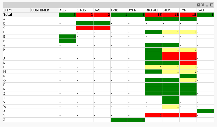
I expanded my example to test the expression and I encountered a problem with the sorting of my customers.

I would like the customers to be served according to the registration date. That means I sort the customers in the pivot table by registration date ascending.

Now, in my example Michael, Steve and Tom registered on the same date. So in that case I'd like to serve them alphabetically.

That is why in the sorting tab I sort customer by expression 'Registration_Date' ascending and alphabetically A -> Z.

And there the expression doesn't work anymore.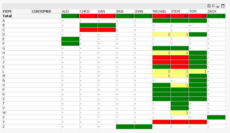

For example: Have a look at item K, two of them are in the warehouse, and I would like Michael and Steve to have it, but here Micheal and Tom get one.

I guess that is because Tom and Michael are loaded first in the inline table.

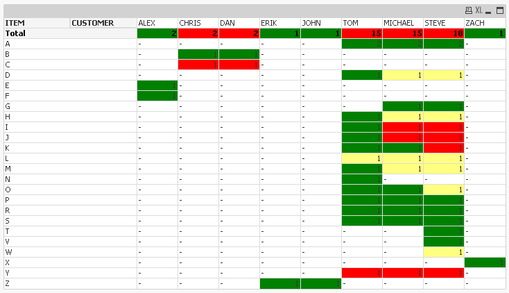
If I don't sort alphabetically, Tom, Michael and Steve appear in the pivot table in the order they were loaded in the inline table in the script and everything works fine:

[sunny_talwar]

I am going to break my response into two parts since the response to first part is fairly quick and I will need to spend some more time on the second part.

So, to answer you first question, you are absolutely right that we usually need to use Before or After function for a pivoted column of a pivot table. But when you use an Aggr table (even when using the pivot table) the imaginary table that the function creates, it doesn't create a pivot table. So, essentially Aggr() function is creating a straight table where all columns are still columns and nothing is pivoted. So when we use Aggr(), Before and After doesn't work and you need to use Above and Below() instead.

I hope this make sense.

Best,

Sunny

[sunny_talwar · Accepted solution]

Does this look right?

If it does, then I hope you have QV12 or above installed because there is a solution available in QV12 which can resolve your problem without making any changes in the script. (The sortable Aggr function is finally here!‌. QV12 came up with a new way to sort in ascending or descending order within Aggr() function which was not available previously. Previously, Aggr() only sorted in the load order. So, if you don't have to have QV12, you will need to fix your load order for customer in the script.

Expression for color:

=Pick(Max(Aggr(If(sum(ORDER_AMOUNT) > 0,

If(ORDER_AMOUNT + If(RangeSum(Above(Sum(ORDER_AMOUNT), 1, RowNo())) > 0, RangeSum(Above(Sum(ORDER_AMOUNT), 1, RowNo())), 0) <= WAREHOUSE_AMOUNT, 1,

if(ORDER_AMOUNT + If(RangeSum(Above(Sum(ORDER_AMOUNT), 1, RowNo())) > 0, RangeSum(Above(Sum(ORDER_AMOUNT), 1, RowNo())), 0) <= WAREHOUSE_AMOUNT + SHIPPING_AMOUNT, 2,

3)),

4), ITEM, (CUSTOMER, (TEXT, ASCENDING)))), RGB(0,128,0), RGB(255,255,128), RGB(255,0,0), RGB(255,255,255))

Like I mentioned, if you don't have QV12 or above, you will have to make sure that CUSTOMER are loaded in ascending order. If you do that, then that should fix your issue.

HTH

Best,

Sunny