Unlock a world of possibilities! Login now and discover the exclusive benefits awaiting you.
- Qlik Community
- :
- All Forums
- :
- QlikView App Dev
- :
- Percent of Total in Pivot Table
- Subscribe to RSS Feed
- Mark Topic as New
- Mark Topic as Read
- Float this Topic for Current User
- Bookmark
- Subscribe
- Mute
- Printer Friendly Page
- Mark as New
- Bookmark
- Subscribe
- Mute
- Subscribe to RSS Feed
- Permalink
- Report Inappropriate Content
Percent of Total in Pivot Table
Hello-
I like the Pivot Table functionality because it allows me to drill through to the details in another table. A straight table allows that, but not as well in my example. Mainly because I need two dimensions.
I have included in the attached doc some options.
In the end I want a table that looks like this. I can re-model the data if needed so I am open to any suggestions.
| Yes | No | Total | %Yes | |
| Red | 50 | 16 | 66 | 76% |
| Orange | 57 | 62 | 119 | 48% |
| Black | 30 | 18 | 48 | 63% |
| Green | 98 | 38 | 136 | 72% |
When I click on the 16 for No/Red I would like to just see those 16 detail records. While I can get a straight table to look the way I want, I can not get it to select the data I want (Because I am using Set Analysis instead of the Dimension as a Dimension in the chart)
- « Previous Replies
-
- 1
- 2
- Next Replies »
Accepted Solutions
- Mark as New
- Bookmark
- Subscribe
- Mute
- Subscribe to RSS Feed
- Permalink
- Report Inappropriate Content
Check out the attached
Script:
LOAD Color,
Sentiment,
ID
FROM
Percent.xlsx
(ooxml, embedded labels, table is Data);
LOAD * Inline [
DIM
1
2
3
];
Pivot Table
Dimensions
1) Color
2) =Pick(DIM, Sentiment, 'Total', 'Percent')
Expression
=Pick(DIM, Count(ID), Count(ID), Num(Count({$<Sentiment={'Yes'}>}ID)/Count(ID), '##.%'))
Sort Expression for 2nd dimension
=Match(Pick(DIM, Sentiment, 'Total', 'Percent'), 'Yes', 'No', 'Total', 'Percent')
- Mark as New
- Bookmark
- Subscribe
- Mute
- Subscribe to RSS Feed
- Permalink
- Report Inappropriate Content
Thanks, that works well.
- Mark as New
- Bookmark
- Subscribe
- Mute
- Subscribe to RSS Feed
- Permalink
- Report Inappropriate Content
where is your Percent.xlsx. I am not getting this without it.
- Mark as New
- Bookmark
- Subscribe
- Mute
- Subscribe to RSS Feed
- Permalink
- Report Inappropriate Content
Here you go 
Note: I just exported the table box with the three fields and saved it as Percent.xlsx
- Mark as New
- Bookmark
- Subscribe
- Mute
- Subscribe to RSS Feed
- Permalink
- Report Inappropriate Content
This pivoting I know Sunny. We can do it only in Pivot table. But using Pivot, it is not possible every time for merging like below,
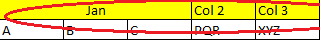
What is best practice in that case?(Suggestions) - Splitting Col 2,Col 3 in different report?
- Mark as New
- Bookmark
- Subscribe
- Mute
- Subscribe to RSS Feed
- Permalink
- Report Inappropriate Content
If you can provide some mock up data (in Excel) and provide the expected output, I might be able to help you out
- Mark as New
- Bookmark
- Subscribe
- Mute
- Subscribe to RSS Feed
- Permalink
- Report Inappropriate Content
See I have raw data(Can't share) and one date on which date dimension is dependent. I want your suggestion on the scenario.
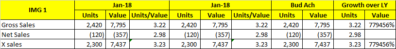
IMG 1 : Complete report
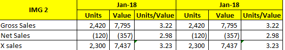
Now, I know using Pivot we can create report like IMG 2
But, in my report there is extra part like (IMG 3 below) with IMG 2 part which I think I can't append with IMG 2 in PIVOT Table.
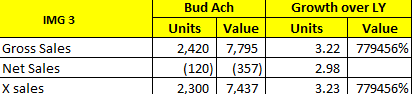
Kindly suggest me about the approch
1> Can we create such report in same table?
2> Is it standard way to split the report(IMG 1) into 2 reports (IMG 2, IMG 3)?Because by splitting them I think we can develop it.
- Mark as New
- Bookmark
- Subscribe
- Mute
- Subscribe to RSS Feed
- Permalink
- Report Inappropriate Content
I am unable to load images, would you be able to post the Excel file for me
- Mark as New
- Bookmark
- Subscribe
- Mute
- Subscribe to RSS Feed
- Permalink
- Report Inappropriate Content
Ok let me start a discussion.
- « Previous Replies
-
- 1
- 2
- Next Replies »