Set Analysis - Exclude Rows Based on Aggregate / Expression

[#1]

I want to create a simple chart (pivot table) with two expressions:

count(ID)

sum(Weight)

But I only want to display items which have count(ID) > 1.

Can I do that with set analysis?

I know in SQL it would be a simple "HAVING count(ID) > 1" clause with a group by but I can't figure out how the syntax for set analysis.

I suspect it's pretty simple but I just don't get the set analysis.

Any help would be greatly appreciated.

[MayilVahanan]

Hi,

Try this,

=If(Count(ID) > 1, Sum(Weight), 0)

Hope it helps

[#3]

I do not want that column to show zero, I do not want those items in the chart (straight table) at all.

[MayilVahanan]

Hi,

See the attached file.. Hope it helps

[#5]

I think you are still misunderstanding. I want the data fields that I had already to show on the chart. I just want the row with count(ID)  equal to 1 to NOT be displayed at all.

Your formula managed to hide that row, but somehow your version does not have the count(ID) and sum(Weight) fields anymore. When I add them back into your version, the line with count(ID) shows back up with a null in your new field.

[#6]

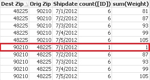
I just do not want the row in red in the table at all...

[#7 · Accepted solution]

This turned out to be a matter of simply putting the IF criteria on ALL my expressions. That caused all the expressions in the table to end up being null, thereby causing QlikView to hide the entire row.

Thank you Mayil Vahanan Ramasamy for setting me on the right track.

Sue