Sorting in Pivot table

[#1]

Guys,

I have a pivot table like :

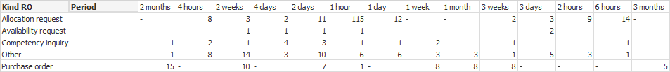
I need to sort this table like 1 hour, 2 hours, 4 hours, 1 day......, 1 week....., 1 month etc.

I tied like numeric sort and text sort, but it doesnt give me the desired result.

Any ideas?

[robert_mika]

Could you attached your file?

[rubenmarin]

Hi Diana, you can use Dual() function when you're creating your Period values, this way you can sort Period dimension by number.

In example:

If(Minutes<60, Dual('1 hour', 1),

If(Minutes <120, Dual('2 hours', 2),

  If(Minutes <240, Dual('4 hours', 3)... and so on.

[#4 · Accepted solution]

I've solved this problem using : =match([Period],'1 hour','2 hours','4 hours','6 hours','1 day', '2 days', '3 days', '4 days','1 week', '2 weeks', '3 weeks', '1 month', '2 months', '3 months')

in sort---> Expression