Weighted average

[#1]

Hi all, need some help please in calculating the weighted average, for this contrived example I have 2 figures which are in a Pivot table, in  the following format (one fact table), lets say one figure represents the count of sales and the another figure represents the average time of those sales per department.

How can I calculate the weighted average time of sales of each different product for a company (i.e. not by department)???

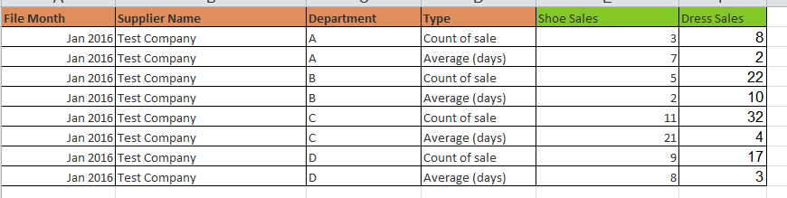
I've tried something like this but I think I need to use the AGGR function but not quite sure how.

=SUM(({$<Type={"Count of sale"}>}[Shoe Sales]) * ({$<Type={"Average (days)"}>}[Shoe Sales]))/SUM({$<Type={"Count of sale"}>}[Shoe Sales])

Many thanks in advance!

[sunny_talwar · Accepted solution]

May be this:

Sum(Aggr(Only({<Type = {'Count of sale'}>} [Shoe Sales]) * Only({<Type = {'Average (days)'}>}[Shoe Sales]), [File Month], [Supplier Name], Department))/Sum({<Type = {'Count of sale'}>} [Shoe Sales])

[#3]

Many thanks for this, works perfectly, I was actually trying it with Only instead of Sum but was missing the AGGR bit, thanks again!

[sunny_talwar]

Awesome