Different color for each subtotal-line

[Anonymous]

Hello all,

I have a table, currently looking like this:

I managed to get the 1st Total-line 'isolated' using rowno() so I can give it a separate color (choose yellow now to make it stand out).

I managed to get the 3rd Total-line 'isolated' using Dimensionality() so I can do the same (choose green to match the dimension)

Now, how do I 'isolate' the 2nd Total-line? I only managed to 'isolate' the entire block using a combination of both Dimensionality() and rowno(), but I can't seem to 'isolate' the Total-line so I can color it.

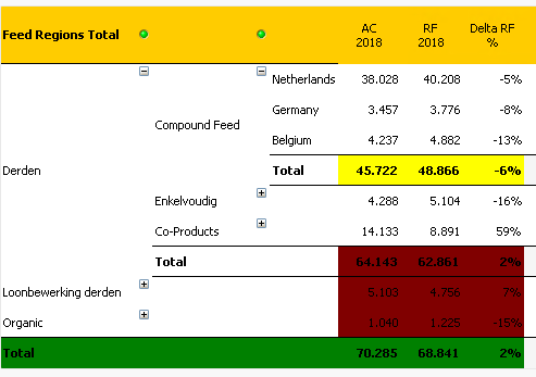
What I want, is that only the Total-line gets the red color, the other two lines should become white.

The formula used on the 3 expression-columns for the color is this:

=if(rowno()=0,yellow(),if(Dimensionality()=0,green(),if(Dimensionality()=1,if(isnull(rowno()),red(),white()),white())))

Anyone got any ideas?

Thanks in advance for any suggestions!

[marcus_sommer · Accepted solution]

As far as your dimension-values are always sorted in the same way you could try it with dual-values of them like:

dual(FIELD, autonumber(FIELD)) as FIELD

It just required that you order the fieldvalues in the wanted way. An alternatively to the autonumber() might be a pick(match()) or an applymap() matching.

If your pivot is dynamic in any way the above method won't work. In this case you need to rank your dimension-values in some way - either per an applied numeric sorting or with a ranking on the dimension-values itself. Here an example in which direction it might go:

avg(aggr(NODISTINCT num(rank(total MaxString([FIELD]), 1)), [FIELD]))

and this could be wrapped with a pick(match()) to assign the colors to the rank-position (this also menat for the dual-example from above).

Beside this are you sure that you really want to make the table so colorful? IMO it doesn't help the readability of the content.

- Marcus

[njmaehler]

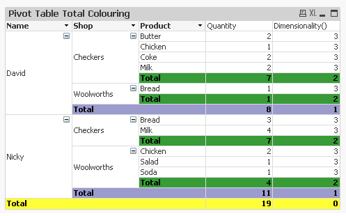
Hi Stefan,

You should be able to achieve this with Dimensionality() and Background Color

I added was the following code to all the Dimensions and Expressions (by clicking on the little plus sign next to the field name) then under the Background Color option:

=if(Dimensionality() = 0, yellow(200),

          if(Dimensionality() = 1, blue(100),

               if(Dimensionality() = 2, green(200),

                    white()

               )

          )

)

You can select any color you want via the rgb(?,?,?) options too.

[Anonymous]

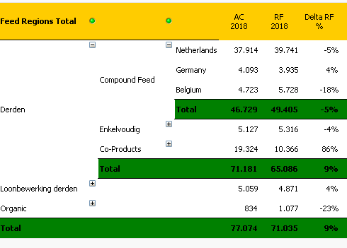
Thanks marcus_sommer, the dual-function in the script worked like a charm, since my Dimension order is always the same indeed. I agree on the 'so colorful' remark by the way, only made the colors stand out in my example to clarify things - see the image below for the end-result .

Might anyone else need this in the future, here's what I did:

I added

dual([Feed Regions Total],AutoNumber([Feed Regions Total])) as DUALFIELD

to my script and used that to create the following Background Color Formula:

=if(rowno()=0,green(),if(Dimensionality()=0,green(),if(Dimensionality()=1,if(DUALFIELD='Derden',green(),white()),white())))

Gave me this as end-result:

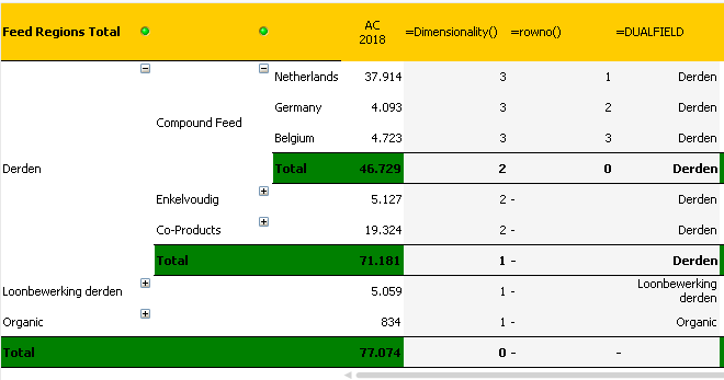
Another image, showing the values for Dimensionality(), rowno() and DUALFIELD which helped create the color-formula: