Different colour of lines in pivot tables

[#1]

Hello All,

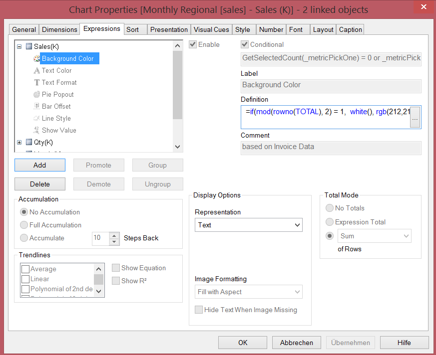
I usually use this expression to make 1 line white and 1 line grey in my normal table:

=if(mod(rowno(TOTAL), 2) = 1,  white(), rgb(212,212,212))

However, it is not working in a pivot table.

Any idea why I do not get the same result on my pivot table.

Many Thanks,

Hasvine

[Anonymous]

Hello Hasvine,

can you post example. I have a Pivot table with your Expression and it works

[jonas_rezende]

Hi,Hasvine Dhurmea.

Make the following steps below:

Click-right and choice Properties...

In Dimension tab

1. Expand ( + ) Dimension , in Background Color put expression.

if(Dimensionality()> 0,

  if(mod(rowno(TOTAL), 2) = 1,  white(), rgb(212,212,212))

)

2. Click Ok.

In Expression tab

1.Expand ( + )  Expression, in Background Color put expression.

if(Dimensionality()> 0,

  if(mod(rowno(TOTAL), 2) = 1,  white(), rgb(212,212,212))

)

2. ClickOk.

Hope this helps.

[#4]

Hi Rudolf,

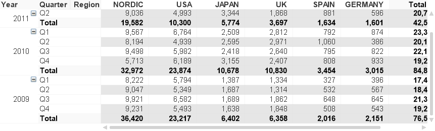
Below is the screenshot.

Many thanks for your help.

KR,

Hasvine

[#5]

No luck,

It does not colour 1 line white and 1 grey.

The first 2 lines are white and the third lines become grey and 7 line become white and the last two lines become grey.

😞

Kind Regards,

Hasvine

[Anonymous]

Hi Hasvine

I defined the Color under Expression. Yours also?

[#7]

Yes i defined the colour in both the dimension and the expression but still no success.

[qlikviewwizard]

‌hi,

please check this link:

Colors based on salaries

[Anonymous]

can you post small sample? only your Chart?

[jonas_rezende]

Hasvine Dhurmea.

Remove Dimensionality() function of the expression, after appropriating their Pivot Table. Ex.:

if(mod(rowno(TOTAL), 2) = 1,  white(), rgb(212,212,212))

Regards,

Jonas Melo.