Expression first record calculation differs from subsequent calculations - how to?

[#1]

Hi,

In many spreadsheets or scenarios - such as calculating exponential weighted moving averages and the like one has an initialisation calculation which is then used as input into subsequent calculations, but since the first calculation in the series has no previous cell to refer to (like in a spreadsheet) one does a different calculation on that first cell and then the rest of the cells in that column/row use the final actual desired calculation for the rest of the data.

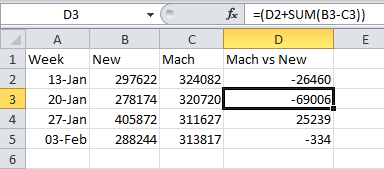
e.g. in a simple spreadsheet

Cell D2 calculation is B2 - C2 , i.e. 297422-324082

Cell D3 calculation is D2 + SUM(B3-C3)

Cell D4 calculation is D3+SUM(B4-C4)

etc

i.e. the Cell D2 calculation is different from the rest in column D

Obviously in Excel its easy,

In QV I've imported columns A,B,C via a script and can do the column D calc either within a script of as an expression in a chart. I trying to use the expression in the chart, i.e. =[New]-[Mach] but I need the expression to change to look up the previous value, and then I discovered never mind just that how do I actually get 2 different calculations into the same expression for different records.

I'm thinking possibly with a nested IF where it checks if record(1) then do calc A and if record > 1 then do calc B which revers to the value of the previous record but am unsure of the correct syntax or optimal approach.

Can anyone shed some light with a worked example please. Thanks

[#2 · Accepted solution]

The way I was able to implement this in the script was by using the peek function.  When reloading the script the peek function will look at the previous field's value in the data.

Since I don't have the original excel spreadsheet I created an inline table similar to the data set above.

test:

LOAD * INLINE [

Order, New, Mach

1, 297622, 324082

2, 278174, 320720

3, 405872, 311627

4, 288244, 313817

]

;

test2:

LOAD *,

New - Mach as Calc

Resident test;

Drop table test;

test3:

LOAD *,

IF (rowno() = 1, Calc, IF (rowno() >= 2, peek([New vs Mach]) + Calc)) as [New vs Mach]

Resident test2;

Drop table test2;

So the basic idea is create a field called Calc that does the basic New-Mach equation.

Then create the New vs Mach field, for the first row just use the Calc field like you mentioned earlier, but if its the second row or above you need to use peek([New vs Mach]) + Calc.

This produces the same results as what you got in excel (for me at least).

Hope this helps...

-Brandon

[#3]

Hi Brandon,

Fantastic! Your solution works 100% for me. Thanks very much for a brilliant answer.