The Above Function - Qlik Community

hic · ‎2015-10-27

The Above() function is a very special function. It is neither an aggregation function, nor a scalar function. Together with some other functions, e.g. Top(), Bottom() and Below(), it forms a separate group of functions: Chart inter-record functions. These functions have only one purpose: To get values from other rows within the same chart.

The basic construction is the following:

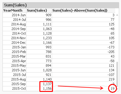
Above( Sum( Sales ) )

This will calculate the sum of sales, but for the row above.

The most common use case is when you want to compare the value of a specific row with the value of the previous row; e.g. this month’s sales compared to last month’s sales.

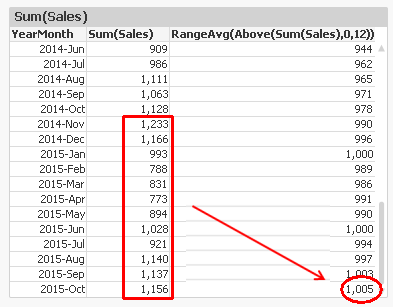
Another use case is when you want to calculate rolling averages. Then you need to use the second and third parameter; the offset and the number of cells. Below, I use

Above( Sum( Sales ), 0, 12 )

The function will return 12 rows: the value for current row and the 11 rows above. This means that you need to wrap it in a range function in order to merge all values to one value. In this case, I use RangeAvg() to calculate the average of the 12 rows.

However, both the above solutions have a flaw: They don’t take excluded values into account. For example, if April is excluded due to a selection, the previous month of May becomes March, which probably isn’t what you want.

To correct this, you need to make the chart show all months, also the excluded ones. In QlikView, you have a chart option “Show all values” that you can use. A method that works also in Qlik Sense, is to add zero to all values, also for the excluded dimensional values:

Sum( Sales ) + Sum( {1} 0 )

Make sure to “Show zero values”.

You can also use the Above() function inside an Aggr() function. Remember that the Aggr() produces a virtual table, and the Above() function can of course operate in this table instead. This opens tremendous new possibilities.

First, you can make the same calculations as above, by using

Only(Aggr(Above(Sum({1} Sales)), YearMonth))

Only(Aggr(RangeAvg(Above(Sum({1} Sales),0,12)), YearMonth))

Note the Set Analysis expression in the inner aggregation function. The {1} ensures that all values in the virtual table are calculated, so that the Above() function can fetch also the excluded ones. Using {1} is maybe too drastic – it is often better to use a Set expression that clears only some fields, e.g. {$<YearMonth=>}.

Further, you can have a virtual table that is sorted differently from the chart where the expression is displayed. For example, the expression

Aggr(Above(Sum(Sales)),Year,Month)

displays the value from the previous month from the same year. But if you change the order of the dimensions, as in

Aggr(Above(Sum(Sales)),Month,Year)

the expression will display the value from the same month from the previous year. The only difference is the order of the dimensions. The latter expression is sorted first by Month, then by Year. The result can be seen below:

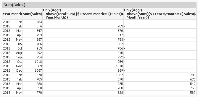
An Aggr() table is always sorted by the load order of the dimensions, one by one. This means that you can change the meaning of Above() by changing the order of the dimensions.

With this, I hope that you understand the Above() function better.

HIC