Unlock a world of possibilities! Login now and discover the exclusive benefits awaiting you.
- Qlik Community
- :
- All Forums
- :
- QlikView App Dev
- :
- Re: Conditionnal Formatting
- Subscribe to RSS Feed
- Mark Topic as New
- Mark Topic as Read
- Float this Topic for Current User
- Bookmark
- Subscribe
- Mute
- Printer Friendly Page
- Mark as New
- Bookmark
- Subscribe
- Mute
- Subscribe to RSS Feed
- Permalink
- Report Inappropriate Content
Conditionnal Formatting
Hi everybody 😎,
I want in a chart to show a conditionnal formatting for some values like this .
If A - B > 0, then show a green arrow
If A = B, then show a gray arrow
If A - B < 0, then show a red arrow
I've seen the image of the arrow and In my chart, i put the formula :
=If(A- B > 0, 'qmem://<bundled>/BuiltIn/arrow_n_g.png', 'qmem://<bundled>/BuiltIn/arrow_e_r.png')
But it doen't work 🙄
Anybody has a idea ?
Accepted Solutions
- Mark as New
- Bookmark
- Subscribe
- Mute
- Subscribe to RSS Feed
- Permalink
- Report Inappropriate Content
Hi
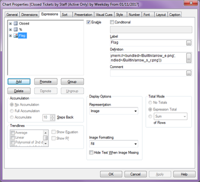
You need to set Representation to "Image" and Image Formatting to Fill as below
Hope this helps
Cheers
Adrian
- Mark as New
- Bookmark
- Subscribe
- Mute
- Subscribe to RSS Feed
- Permalink
- Report Inappropriate Content
Hi Fanch,
have you tried something like
IF(Sum(A-B) > 0, 'qmem://<bundled>/BuiltIn/arrow_n_g.png', 'qmem://<bundled>/BuiltIn/arrow_e_r.png')
Also expression must be represented as "Image".
Pls see image attached
- Mark as New
- Bookmark
- Subscribe
- Mute
- Subscribe to RSS Feed
- Permalink
- Report Inappropriate Content
Hi
Try the following
=IF(Sum(A-B) > 0,'qmem://<bundled>/BuiltIn/arrow_n_g.png',
If(Sum(A-B) = 0,'qmem://<bundled>/BuiltIn/arrow_w.png',
'qmem://<bundled>/BuiltIn/arrow_e_r.png'))
Also as stated above make sure the expression is set to Image and you may have to change the Image Formatting option to get a decent image.
Regards
Adrian
- Mark as New
- Bookmark
- Subscribe
- Mute
- Subscribe to RSS Feed
- Permalink
- Report Inappropriate Content
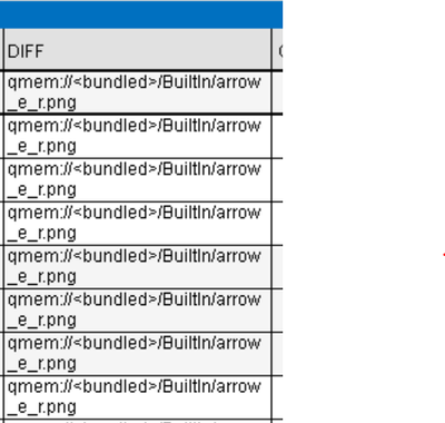
Yes, i've tried this solution. but instead of putting my arrows doing by conditionnal formatting, i have the formula like a string characters 😲
- Mark as New
- Bookmark
- Subscribe
- Mute
- Subscribe to RSS Feed
- Permalink
- Report Inappropriate Content
Hi
You need to set Representation to "Image" and Image Formatting to Fill as below
Hope this helps
Cheers
Adrian
- Mark as New
- Bookmark
- Subscribe
- Mute
- Subscribe to RSS Feed
- Permalink
- Report Inappropriate Content
Yeaaah !!!
Greats,
Thanks a lot ! 🍺
- Mark as New
- Bookmark
- Subscribe
- Mute
- Subscribe to RSS Feed
- Permalink
- Report Inappropriate Content
Hi
Glad to be a help.
So that this helps others please mark the solution as correct.
Cheers
Adrian

