Unlock a world of possibilities! Login now and discover the exclusive benefits awaiting you.
Announcements
ALERT: QlikView server communication interruptions following Microsoft Windows Domain Controller security updates
- Qlik Community
- :
- Support
- :
- Support
- :
- Knowledge
- :
- Member Articles
- :
- Select Top Ranks from QlikView and Use Them With C...
Options
- Move Document
- Delete Document
- Subscribe to RSS Feed
- Mark as New
- Mark as Read
- Bookmark
- Subscribe
- Printer Friendly Page
- Report Inappropriate Content
Select Top Ranks from QlikView and Use Them With Custom Excel Formulas
Turn on suggestions
Auto-suggest helps you quickly narrow down your search results by suggesting possible matches as you type.
Showing results for
Employee
- Move Document
- Delete Document
- Mark as New
- Bookmark
- Subscribe
- Mute
- Subscribe to RSS Feed
- Permalink
- Report Inappropriate Content
Select Top Ranks from QlikView and Use Them With Custom Excel Formulas
Last Update:
Nov 25, 2015 9:37:06 AM
Updated By:
Created date:
Nov 25, 2015 9:37:06 AM
You will learn how to create a chart using a defined range of rows from a QlikView chart object in this tutorial. Avoid table expansion invalidating cell references in custom Excel formulas.
Create New Excel Report
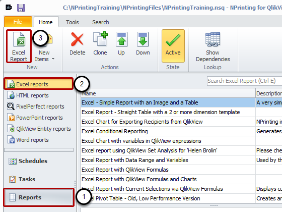
- Select Reports in the lower left pane
- Select Excel reports in the upper left pane
- Select Excel Report in the New group of the function ribbon
Name Report and Create New Template
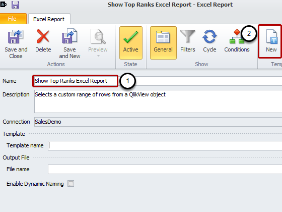
- Enter Show Top Ranks Excel Report as Name for your report and optionally a Description
- Select New in the Template group
Open Select Objects Window
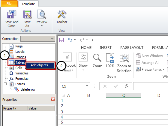
- Right click on the Tables node
- Click on Add objects
Select Object
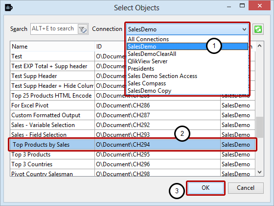
- Select the Connection to the QlikView document that contains the object that you want, SalesDemo in this case
- Select Top Products by Sales - CH294
- Click on the OK button
Adjust Table Properties
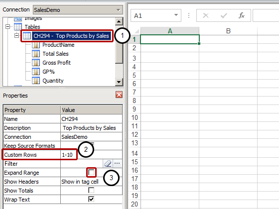
- Make sure CH294 - Top Products by Sales is selected
- Enter the row range you want to import in the Custom Rows field
- Unflag the Expand Range Option
Drag Your Chart into Template
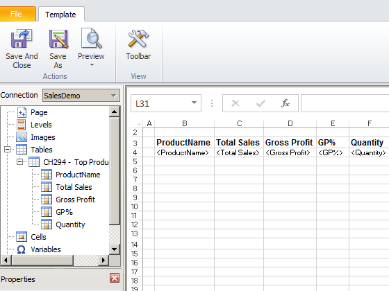
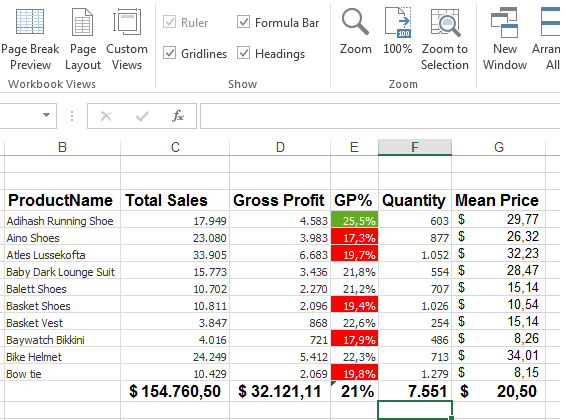
Drag your chart columns into the template. Make sure that there are at least 10 blank rows above the chart.
Mean Price Formula
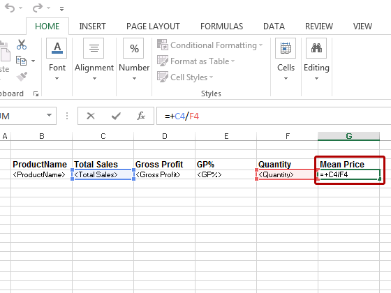
We are going to add a new column to calculate the mean price. We will use a simple formula that refers to the value in specific cells.
- Enter the Mean Price column heading
- Enter the formula to calculate the mean price
Expand Formula
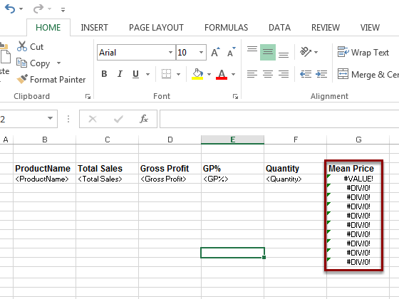
Expand the formula in the Mean Price column for 10 rows
Format Mean Price
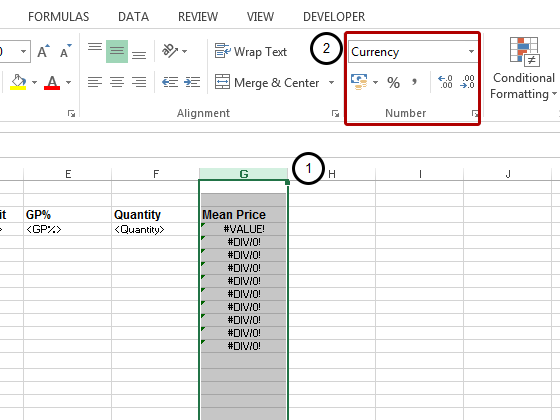
- Select the Mean Price Column
- Format the column as Currency
Add Gross Profit Total
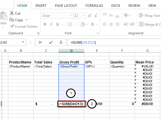
- Select the 10th cell under the Gross Profit Sales heading.
- Enter the formula to calculate Total Sales. Note that you don't need to leave a blank row since NPrinting will not expand the table
- Format the total cells as you prefer
Choose Correct Format
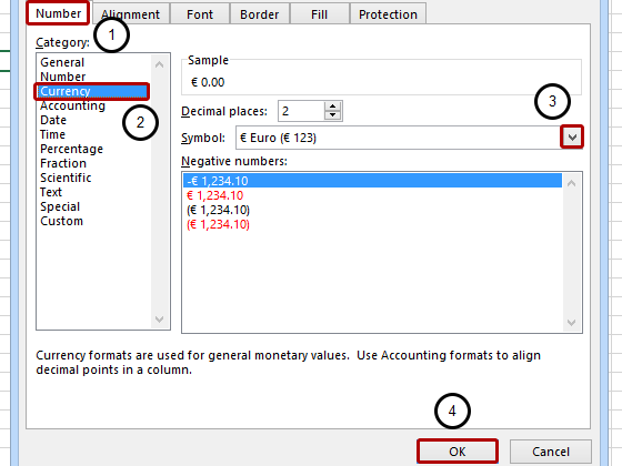
- Select Number
- Choose Currency in the category table
- Choose the symbol you need from the Symbol menu
- Click OK
- Add formatted totals also for "Total Sales" and for "Quantity"
Add GP% Formula
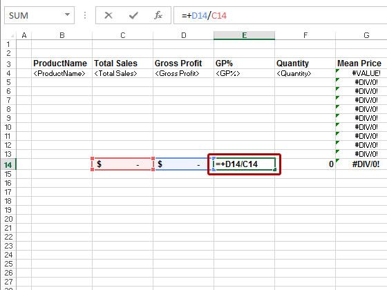
- Select the 14th cell under the GP% column heading.
- Enter the formula to calculate the mean GP%
Format Mean GP%
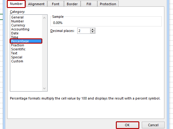
- Right click on the cell containing the mean GP% formula
- Choose Format Cells.... The Format Cells window opens
- Select Number
- Choose Percentage in the category table
- Click OK
Preview
Click Preview in the template ribbon bar