Unlock a world of possibilities! Login now and discover the exclusive benefits awaiting you.
- Qlik Community
- :
- Forums
- :
- Analytics
- :
- App Development
- :
- Re: Comparing values across all columns in pivot t...
- Subscribe to RSS Feed
- Mark Topic as New
- Mark Topic as Read
- Float this Topic for Current User
- Bookmark
- Subscribe
- Mute
- Printer Friendly Page
- Mark as New
- Bookmark
- Subscribe
- Mute
- Subscribe to RSS Feed
- Permalink
- Report Inappropriate Content
Comparing values across all columns in pivot table.
Hi,
I've got the following pivot table:
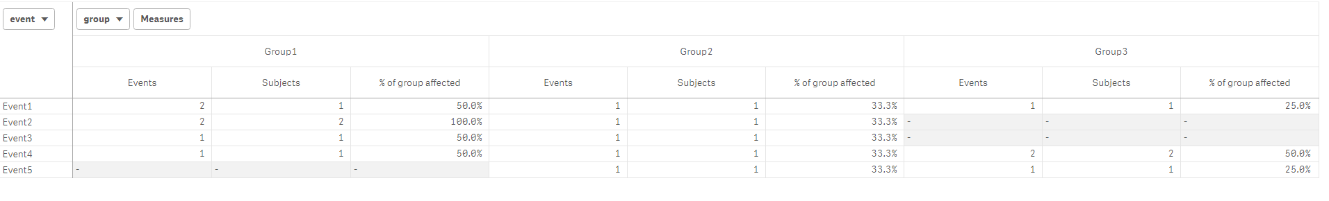
What I'd like to do is...
...for each row, compare the "%of group affected" value for each Group and if the difference between the highest and lowest "% of group affected" is >= 50, set the background color of the highest "%of group affected" in the row to yellow.
I already know how to calculate "%of group affected" and how to identify when a cell contains the highest or lowest value by using hrank().
What I need is an expression I can use when specifying a cell's background color that will calculate the difference between highest and lowest "%of group affected" in the row. I tried using the rangemax() and rangemin() with before() and after() functions but I couldn't get them to work.
Thanks,
Steve
- Mark as New
- Bookmark
- Subscribe
- Mute
- Subscribe to RSS Feed
- Permalink
- Report Inappropriate Content
well this works, but I wonder if there's a better way....
=rangemax(before(count(distinct subject)/Aggr(NODISTINCT Count(DISTINCT subject), group),0,ColumnNo()),after(count(distinct subject)/Aggr(NODISTINCT Count(DISTINCT subject), group),0,noofcolumns()-columnno()+1))
-rangemin(before(count(distinct subject)/Aggr(NODISTINCT Count(DISTINCT subject), group),0,ColumnNo()),after(count(distinct subject)/Aggr(NODISTINCT Count(DISTINCT subject), group),0,noofcolumns()-columnno()+1))