Create a new measure based on specific combinations of dimensions in a pivot table

[Simona]

Hi guys,

I need your help in finding a solution for the following issue:
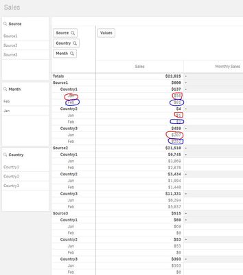
I have a chart that displays Sales by Sources, Countries, and Months (all being filters as well).
I need another measure (Monthly Sales) to display in each row the values of total sales for that month for all countries from that source, like to see in each row the sales for a country (in Sales column) and the sales from all countries in that month (in Monthly Sales column)

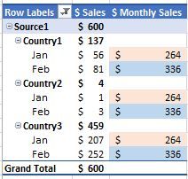
e.g. from below example, in Source 1, in January (marked in red), I should have for Monthly Sales (sum of sales for all countries) = $56+$1+$207= $264, and for February (marked in blue) = $81+$3+$252= $336.

I could easily get this in Excel by creating a new column in the raw data table, with =SUMIFS([Sales],[Source],[@Source],[Month],[@Month]), then inserting a pivot table and get those values:

I've tried this: if(dimensionality()=3,sum (all{<Country=p(Country)>}Measure1)), but I get the correct number just when i filter a source and a month 😞

*Please note that switching dimensions order is not a valid solution for my situation (even if I'll get the values I need) because i need this structure (Source, Country, Month) and i have other measures to calculate.

Kind regards,
Simona