Incorrect average in totals line for pivot table

[mikegrattan]

I'm using the following formula:

Avg(Aggr(Count(Distinct CaseNumber), Warehouse,Year,Date))

The pivot table comes out like this:

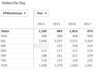
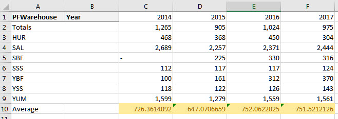
When I try to validate the totals line in Excel, I am getting different numbers:

I am currently hiding Nulls in this table for Warehouse.  PFWarehouse is a calculated master dimension:

=If(Match(Warehouse,'HUR','SAL','SSS','SBF','YUM','YBF','YSS'),Warehouse,Null())

If I do not exclude Nulls from the pivot table I get the following data:

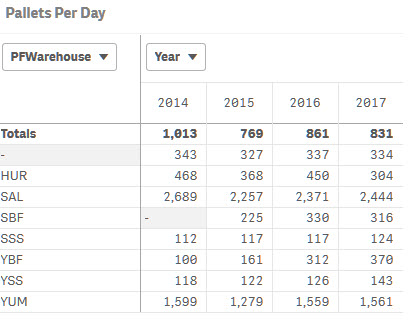
Qlik is adjusting the totals, so I don't think the Null warehouse is throwing this off.  Perhaps my formula needs some fine tuning?

[sunny_talwar]

Date is not one of the dimension, why use it in Aggr() function.... May be this

Avg(Aggr(Count(Distinct CaseNumber), Warehouse,Year))

[mikegrattan]

Date is not in the pivot table, but I want a daily average of pallets per warehouse.

[sunny_talwar]

In that case, I think your row level numbers might not be correct.... you probably should use Avg(Aggr(Count(Distinct CaseNumber), Warehouse,Year,Date)) for your pivot table also

[mikegrattan]

I'm not sure I understand what you're saying.  I am using that formula in my pivot table.  I just don't have the Date dimension showing in my pivot table. 

If I add Date to the pivot table either as a row or a column I am still seeing the same numbers at the row level and in the Totals row.

[sunny_talwar · Accepted solution]

May be try this

Avg(Aggr(Avg(Aggr(Count(Distinct CaseNumber), Warehouse,Year,Date)), Warehouse, Year))

[mikegrattan]

Yes, much better.  Thank you!

[sunny_talwar]

Just better, not perfect

[mikegrattan]

Well...actually it is perfect! 

[sunny_talwar]

I am glad it worked out