Pivot Totals Issues

[RighettiAndrea]

Hi everyone,

I have some issues with the total row in a pivot table.
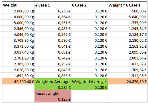
The screenshots I will show, will be taken from an Excel file that I made as an example.

In the total row, I have two weighted averages.
The "€ case 2" is correct because the measure is more simple I think.
The "€ case 1" total result, which is red (0.120 €), is what I get instead of the green one (0.585 €).

Here's my measure (it works fine in the table rows)

How can I fix the measure in order to get the result I want, without affecting the rows of the table?

I hope you understand,

Thank you all!

[jyothish8807 · Accepted solution]

Hi RighettiAndrea,

Can you try aggr and see if it works ? Something like this: or can you share raw sample data instead of snapshot ?

Aggr(Sum(DOC_VEN_Trans),<Your Dimension>)/1000*Aggr(Sum(DOC_VEN_QTA),<Your Dimension>)/Aggr(Sum(DOC_VEN_Trans),<Your Dimension>)

[RighettiAndrea]

Hi,
thank you for your answer!

I've tried with the Aggr function many times but the real issue was with some data in the table that I removed because it was not supposed to be in that analysis.

Anyway, the aggr function was perfect for another issue I had in another measure.

Thank you man!

[jyothish8807]

You are welcome 🙂