Unlock a world of possibilities! Login now and discover the exclusive benefits awaiting you.
- Qlik Community
- :
- Forums
- :
- Analytics
- :
- New to Qlik Analytics
- :
- Re: Dimension for Top 20 Suppliers by Spend and pe...
- Subscribe to RSS Feed
- Mark Topic as New
- Mark Topic as Read
- Float this Topic for Current User
- Bookmark
- Subscribe
- Mute
- Printer Friendly Page
- Mark as New
- Bookmark
- Subscribe
- Mute
- Subscribe to RSS Feed
- Permalink
- Report Inappropriate Content
How to calculate Dimension for Top 20 Suppliers by Spend and per Year in Qlik Sense?
Hi Everyone,
I am trying to create a dimension that calculates the spending of the top 20 suppliers by spend and per year.
My current formula is the following:
=sum({<[Supplier ] = {"=Aggr(Rank(Sum([Spend]))<=20, [Supplier]) "}>} [Spend])I have data between 2019 to 2022 YTD. I use this dimension in a bar chart in which the X-axis shows the Years.
When I select one year, the dimension is calculating the correct figure. However, if I don't select any year, the formula is currently checking the top 20 suppliers for all years and then it checks the spending of these suppliers in each year.
I need that the total spend per year is the same regardless if I select one year or not.
Thanks in advance for your support!
- Tags:
- aggr
- « Previous Replies
-
- 1
- 2
- Next Replies »
- Mark as New
- Bookmark
- Subscribe
- Mute
- Subscribe to RSS Feed
- Permalink
- Report Inappropriate Content
Hi @stevedark
It's the top 20 in each month. The invoices are allocated to months based on their posting date, so I wanted to check the spend of the top 20 suppliers in the spend allocated to each month.
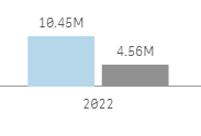
As an example, this is the view for 2022 (the grey bar is the spend on the remaining suppliers, which is obtained by the formula you shared but with ">" instead).
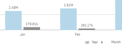
By clicking the bar for 2022, I wanted to see the spend allocated in Jan, Feb, Mar, etc, based on the posting dates of the invoice.
The variation you shared with the tweak to the field is working, but is there a more efficient way of doing it?
Thanks!
Gonçalo
- Mark as New
- Bookmark
- Subscribe
- Mute
- Subscribe to RSS Feed
- Permalink
- Report Inappropriate Content
- Mark as New
- Bookmark
- Subscribe
- Mute
- Subscribe to RSS Feed
- Permalink
- Report Inappropriate Content
Hi @stevedark,
The tweak is the second part of the If. I basically took your suggestion but repeated the first part of the If into the second part and replaced Year by Month.
=if(GetPossibleCount(Year) > 1,
sum(aggr(if(rank(sum(Spend)) <= 20, sum(Spend), null()), Year, Supplier)),
sum(aggr(if(rank(sum(Spend)) <= 20, sum(Spend), null()), Month, Supplier)))
From the testing I did, it is showing the desired result, although I'm not sure if it is the optimal way.
Best,
Gonçalo
- Mark as New
- Bookmark
- Subscribe
- Mute
- Subscribe to RSS Feed
- Permalink
- Report Inappropriate Content
Hi @Goncalo
It's absolutely fine to do it like that. You could probably make the code slightly less repetitive by doing this:
sum(aggr(if(rank(sum(Spend)) <= 20, sum(Spend), null()), $(=if(GetPossibleCount(Year)>1,'Year','Month')), Supplier))But it is more obvious what is going on with the IF statement on the outside.
Cheers,
Steve
- Mark as New
- Bookmark
- Subscribe
- Mute
- Subscribe to RSS Feed
- Permalink
- Report Inappropriate Content
Thank you @stevedark for all the support!
- Mark as New
- Bookmark
- Subscribe
- Mute
- Subscribe to RSS Feed
- Permalink
- Report Inappropriate Content
Hi @stevedark,
I need to create a variation of this metric when instead of looking at amount of spend of the top 20 suppliers by spend, I want to calculate the % of spend that is coming from the top 20% of suppliers ranked by spend.
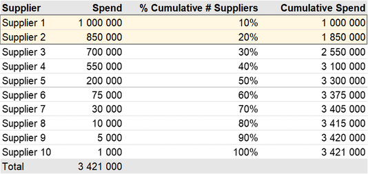
Below I leave a table illustrating my need, assuming that there are 10 suppliers:
The value I need to obtain is the sum of spend of the suppliers that correspond to 20% of the supplier base, i.e. the first two in this example (1M + 0.85M = 1.85M), divided by the total spend: 1.85/3.421 = 54.1%.
I would also need to have this calculation by year, and when selecting one year, I need to be able to see the monthly cumulative evolution of the metric, i.e., in January only data from this month, in February the sum of January + February, etc.
If this is too different to keep it under the original request, I can create a new question in the forum.
Many thanks!
- Mark as New
- Bookmark
- Subscribe
- Mute
- Subscribe to RSS Feed
- Permalink
- Report Inappropriate Content
Hi @Goncalo
There are a few different things to pick up from this question. The first is a percentage, which if we stick with the 20 for now, should be simple as you just divide your limited value by the total:
sum(aggr(if(rank(sum(Spend)) <= 20, sum(Spend), null()), $(=if(GetPossibleCount(Year)>1,'Year','Month')), Supplier))
/
sum(Spend)
In order to have it by the top 20% rather than the top 20, we just need to swap out the number 20 with the correct number. We can calculate this outside of the expression and then inject it in. Using $(= ) allows us to do that.
$(= count(DISTINCT Supplier) * 0.2)If you want to round down the number you can leave that as is (as you are doing a <= anyway) but if you want to include the supplier on the cusp of the 20% you will need to add a ceil function in there also.
So, the percentage for the top 20% of suppliers will be:
sum(aggr(if(rank(sum(Spend)) <= $(= count(DISTINCT Supplier) * 0.2), sum(Spend), null()), $(=if(GetPossibleCount(Year)>1,'Year','Month')), Supplier))
/
sum(Spend)
The accumulation within the year is more interesting. If you are doing it within a table then I would probably recommend having 12 measures and using set analysis to look at just January in the first measure, January and February in the second, etc. Rangesum(Above on both the top 20% and the total and then dividing one by the other may work, but I have found snags with those functions - particularly when there are more dimensions.
Another approach to accumulation is to create a new dimension that does the accumulation for you. This can be done by creating a table that links January in each year to itself and every other month in the year, then February to itself and every subsequent month, through to December which only links to itself. That new dimension can be used as a dimension in a chart and it will accumulate via the associations.
This technique is described in this blog post:
https://www.quickintelligence.co.uk/qlikview-accumulate-values/
Hope that helps,
Steve
- Mark as New
- Bookmark
- Subscribe
- Mute
- Subscribe to RSS Feed
- Permalink
- Report Inappropriate Content
Hi @stevedark
Thanks again for your help and for the detailed explanation!
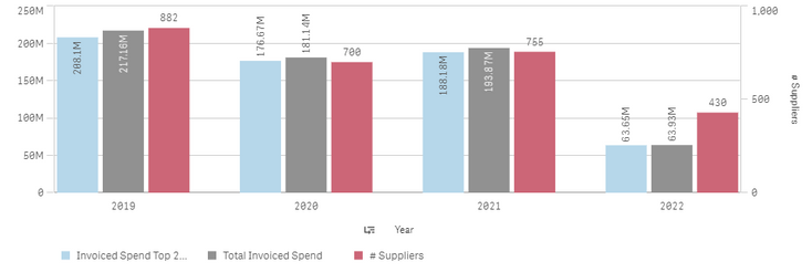
I applied the numerator from the formula above into a bar chart to check the total spend to the top 20% of suppliers. I also add temporarily a new column with just the # of suppliers for troubleshooting.
From what I understood, by injecting the number of suppliers it considers the number of distinct suppliers for the range selected, which distorts the annual figures. Is it possible to change the formula so that it considers the # of top 20% suppliers in each year?
Regarding the cumulative spend per month, which I would like to see by clicking in one of the years above, the last month should be equal to the annual figure. I believe the solution you provided in the link is the best that suits my need.
Should I use as a reference the example you mention in the "Other uses" section?
Many thanks!
Goncalo
- « Previous Replies
-
- 1
- 2
- Next Replies »


