Unlock a world of possibilities! Login now and discover the exclusive benefits awaiting you.
- Qlik Community
- :
- Forums
- :
- Analytics
- :
- New to Qlik Analytics
- :
- Re: Pivot table separate row color
- Subscribe to RSS Feed
- Mark Topic as New
- Mark Topic as Read
- Float this Topic for Current User
- Bookmark
- Subscribe
- Mute
- Printer Friendly Page
- Mark as New
- Bookmark
- Subscribe
- Mute
- Subscribe to RSS Feed
- Permalink
- Report Inappropriate Content
Pivot table separate row color
Hello
I have a pivot table with 2 dimensions - 2 values in first dimension and 3 values in second. That gives me a table with 6 rows. The problem I have to compare (color) each row result with a different target value.
I'm coming from excel, where this was easily done just by referencing a cell value, but being new to qlik, i'm having trouble even figuring out if what i want is even possible.
- Mark as New
- Bookmark
- Subscribe
- Mute
- Subscribe to RSS Feed
- Permalink
- Report Inappropriate Content
Hi @Tadyy ,
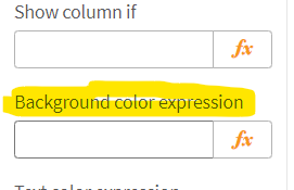
Please try the below-highlighted property of the column where yo can set the expression for the color.
Abhijit
keep Qliking...
Help users find answers! Don't forget to mark a solution that worked for you!
- Mark as New
- Bookmark
- Subscribe
- Mute
- Subscribe to RSS Feed
- Permalink
- Report Inappropriate Content
I've tried that, my issue is what to write inside there. Because it's a pivot table, but I need every row to be colored based on external value that should be specific to that row - I don't know how to identify each specific row with qlik syntax (if that makes sense)
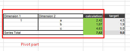
Added what my excel example looks like below
- Mark as New
- Bookmark
- Subscribe
- Mute
- Subscribe to RSS Feed
- Permalink
- Report Inappropriate Content
Hi @Tadyy ,
You can do the same by writing the expression base on your logic.
Abhijit
keep Qliking...
Help users find answers! Don't forget to mark a solution that worked for you!
- Mark as New
- Bookmark
- Subscribe
- Mute
- Subscribe to RSS Feed
- Permalink
- Report Inappropriate Content
well in excel the calculation is part of the pivot, the targets are normal cells that I reference to for the formatting. But how to tell qlik to look basically for 1-a to look at 4,5 and 1-b to look at 5,0...

