Conditional Top 10 values

[#1]

Hello friends,

Please refer to image1 shown above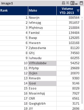

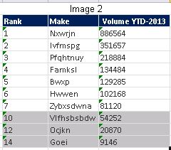
I need to show top 10 values  shown in image2 .Grey color highlighted cells should always be included in top 10.

It would be great if you have some solution for this..

Thanks in advance !!!

[Anonymous]

What logic highlights them in grey ?

[#3]

all 3 highlighted lies in a same brand for ex:-

A11	A
	B
	C

[mohsinqlik]

Dear Snehal,

You can create static variables to find top 7 ranked Make and another 3 variable to find 10,12 and 14th ranked Make and pass them in you those variable in your set analysis expression of volume. This will restrict your dimension to those 10 values. Hope this helps.

Regards,

Mohsin Choudhary

[Anonymous]

Hi,

an example attached.

Can this solution help you?

E

[HirisH_V7 · Accepted solution]

Hi ,

Check this,

=If(MAKE= 'ANT' ,Sum(VOLUME),
If(MAKE= 'BRU' ,Sum(VOLUME),
If(MAKE= 'ROBY' ,Sum(VOLUME),
aggr(if(Rank(Sum(VOLUME))<=10,VOLUME),MAKE))))

In place of the Fields you can place your required fields.

Hope this helps,

PFA,

Hirish

[#7]

Thanks Hirish.. This solution is helpful