Unlock a world of possibilities! Login now and discover the exclusive benefits awaiting you.
- Qlik Community
- :
- All Forums
- :
- QlikView App Dev
- :
- Formating pivot chart
- Subscribe to RSS Feed
- Mark Topic as New
- Mark Topic as Read
- Float this Topic for Current User
- Bookmark
- Subscribe
- Mute
- Printer Friendly Page
- Mark as New
- Bookmark
- Subscribe
- Mute
- Subscribe to RSS Feed
- Permalink
- Report Inappropriate Content
Formating pivot chart
Hi all,
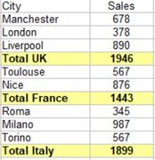
I have two dimensions (country and city) and one expression (sales). What i'am trying to,achieve is the output below (made on Excel).
l can't remember if it's possible with Qlikview. I think it could be esay if we can hide dimension in pivot chart. But we can't![]()
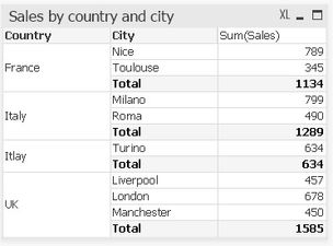
For the moment i get the following chart :
Thanks
Accepted Solutions
- Mark as New
- Bookmark
- Subscribe
- Mute
- Subscribe to RSS Feed
- Permalink
- Report Inappropriate Content
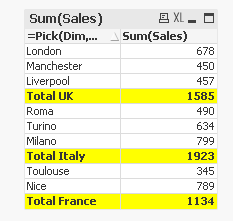
Something like this?
To do this, I created an island table like this in the script
Table:
LOAD * INLINE [
    Country, City, Sales
    France, Nice, 789
    France, Toulouse, 345
    Italy, Milano, 799
    Italy, Roma, 490
    Italy, Turino, 634
    UK, Liverpool, 457
    UK, London, 678
    UK, Manchester, 450
];

Dim:
LOAD * INLINE [
    Dim
    1
    2
];
Now create a straight table like this
Dimension
=Pick(Dim, City, 'Total ' & Country)
Expression
Sum(Sales)
and sort the dimension using this
(Rank(Country)) + Dim/10
Use this for background color of expression and dimension
=If(Dim = 2, Yellow())
and use this for text formatting
=If(Dim = 2,'<b>')
- Mark as New
- Bookmark
- Subscribe
- Mute
- Subscribe to RSS Feed
- Permalink
- Report Inappropriate Content
Hi,
You can get close checking 'Indent Mode' on Style tab & changing the Country dimension to a calculated dimension 'Total ' & Country.
Interested to see if any better suggestions.
Cheers,
Chris.
- Mark as New
- Bookmark
- Subscribe
- Mute
- Subscribe to RSS Feed
- Permalink
- Report Inappropriate Content
Something like this?
To do this, I created an island table like this in the script
Table:
LOAD * INLINE [
    Country, City, Sales
    France, Nice, 789
    France, Toulouse, 345
    Italy, Milano, 799
    Italy, Roma, 490
    Italy, Turino, 634
    UK, Liverpool, 457
    UK, London, 678
    UK, Manchester, 450
];

Dim:
LOAD * INLINE [
    Dim
    1
    2
];
Now create a straight table like this
Dimension
=Pick(Dim, City, 'Total ' & Country)
Expression
Sum(Sales)
and sort the dimension using this
(Rank(Country)) + Dim/10
Use this for background color of expression and dimension
=If(Dim = 2, Yellow())
and use this for text formatting
=If(Dim = 2,'<b>')
- Mark as New
- Bookmark
- Subscribe
- Mute
- Subscribe to RSS Feed
- Permalink
- Report Inappropriate Content
- Mark as New
- Bookmark
- Subscribe
- Mute
- Subscribe to RSS Feed
- Permalink
- Report Inappropriate Content
It works, great Sunny as usual ![]() . Even if i can't understand how the link is made between contry and value 2 of the dim table.
. Even if i can't understand how the link is made between contry and value 2 of the dim table.
- Mark as New
- Bookmark
- Subscribe
- Mute
- Subscribe to RSS Feed
- Permalink
- Report Inappropriate Content
can u pls explain the (Rank(Country)) + Dim/10
- Mark as New
- Bookmark
- Subscribe
- Mute
- Subscribe to RSS Feed
- Permalink
- Report Inappropriate Content
- Mark as New
- Bookmark
- Subscribe
- Mute
- Subscribe to RSS Feed
- Permalink
- Report Inappropriate Content
i agree that it will make sort, but i can't understand,
rank(country) will be 1 2 3
but why adding with DIM/10 can explain deeply pls
example
- Mark as New
- Bookmark
- Subscribe
- Mute
- Subscribe to RSS Feed
- Permalink
- Report Inappropriate Content
Hint: Break the expression and see what it is doing
1) (Rank(Country)) + Dim/10
2) (Rank(Country))
3) Dim/10
and see there values 🙂


