How to change text colour by the condition in pivot table

[#1]

Hello ,

i want to compare with two rows and change the color according to the condition. For example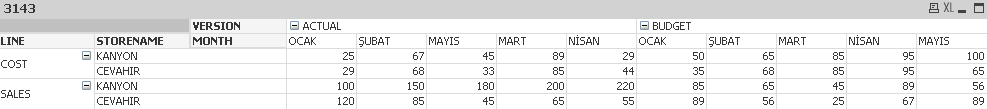

In ACTUAL that i have 25 in Ocak , I want to compare this with BUDGET's Ocak (which is 50). And if it is less than 50 (25<50) it must be red. Then compare with 29 (actual,ocak) vs 50(budget,ocak) and do same things. When it finish , it will come to Subat in ACTUAL then compare with subat in BUDGET then change colour according to my condition. I want to do this with other months(MAYIS , MART , NISAN)

How can i solve it ? I've just started today , so im sorry about my easy question.

[saimahasan]

Do you have only Actual and Budget in version column???

If so then you can easily compare the expression of the two.

If you can provide with the sample data then more accurate solution could be provided.

[MK9885]

Straight Table.

Check the above link.

Right click on the Pivot Table for Custom Format cell and click on what you wanna change, like background or text color and it will be column wise.

You can change the color based on condition.

Note: This will effect the column or to change the color by expression.

If you can upload the test qvw it will be great. If you can;t upload the qvw then maybe your data file (if not confidential) and what requirements.

[vishsaggi]

can you share a sample app please. We need to do use aggr functions like rangesum and before after etc....