How to display column values in colours

[#1]

Hi,

I have a expression in straight table as below

DueDays= = today()-aggr(Date(max(DateDue)),ID)

and the values in that column are

1,975

2,098

1,897

-20

-13

-21

and so on

I would to show The minus values with RED colour and the rest with BLACK. Is this possible?

Thanks.

[jerem1234]

Pie Popout is for Pie charts, here is a snippet from Qlikhelp:

Pie Popout

Click on the Pie Popout in order to enter an attribute expression for calculating whether the pie slice associated with the data point should be drawn in an extracted "popout" position. This type of attribute expression only has effect on pie charts.

Also Text Format can format your text with bold, italic, and underline:

Text Format

Edit the Text Format expression to enter an attribute expression for calculating the font style of text associated with the data point (For tables: text in the table cell for each dimension cell. The calculated text format will have precedence over table style defined in the Chart Properties: Style.) The expression used as text format expression should return a string containing a '<B>' for bold text, '<I>' for italic text and/or '<U>' for underlined text. Note that = is necessary before the string.

Hope this helps!

[#3]

Thanks and this is good.

Suppose if I want to display

$20,£24,£27 and so on in Black colour. and $0 as 'Cancelled'(i, e in text). How can I get this?

[jerem1234]

To represent 0$ as 'Cancelled', you'll need to actually put that into your main expression like:

If(sum(FIELD)=0, 'Cancelled', sum(FIELD))

Then if you want only positive values black, negative red, put the expression into text color:

IF(FIELD<0, rgb(140,0,0), black())

Hope this helps!

[#5]

Yes you are right. Thanks

[#6]

To change Text Format: I changed the Text Format But I haven't observed corrct expected change. can you please post some screens please

[jerem1234]

Bold:

='<B>'

Italic:

='<I>'

Underline:

='<U>'

[#8]

That's really good thanks very much.

Can I ask in the same thread. I have Student Names from A to Z. Is it possible to change the colurs of the names starting with A as Green , B as Black and so on. I tried but semms not showing correct.

[#9]

I used the below in dimension

=If(StudentName='A%',Green())

[jerem1234]

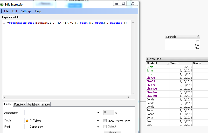
You can use a formula like:

=pick(match(left(Student,1), 'A','B','C'), black(), green(), magenta())

or wildmatch:

=pick(wildmatch(Student, 'A*','B*','C*'), black(), green(), magenta())

Hope this helps!

[#11]

Really Good!!!!!!