Pivot Table

[Anonymous]

Hi guys,

I have a pivot table but what I would like to do is put the sizes along the top and sum the physical and the free columns per size

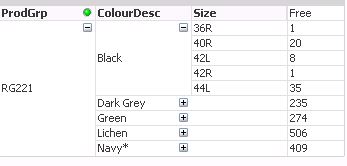
I would like the output to look like this

30S     40R     42L     42R     44L

1          20       8        1         35

Is this possible with the expression somehow?

Thanks!

[Gysbert_Wassenaar · Accepted solution]

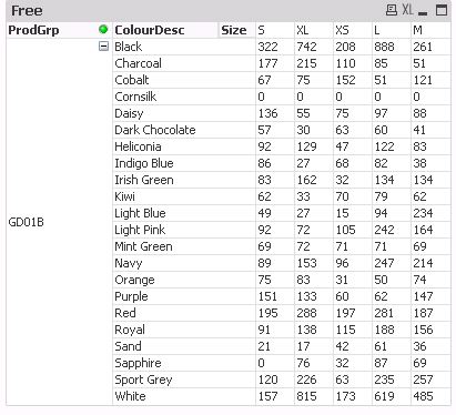
Drag the Size header to the right and just above the expression. When you see a horizontal blue line let go and the Size dimension should be pivoted like you want.

[Anonymous]

Amazing.  Who knew it was something so simple!

Thanks Gysbert

[Anonymous]

Hi guys,

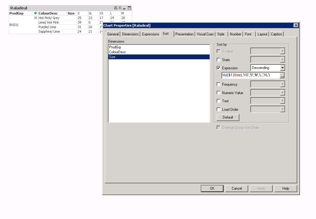
Would you happen to know how to sort the size from S to XL on the top row

Thanks!

[Gysbert_Wassenaar]

Sort that dimension by this expression: =match(only({1}Size),'XS','S','M','L','XL')

[Anonymous]

I tried that but it didn't work..

Thanks a lot for your help so far though

[Gysbert_Wassenaar]

Oops, typo. Change {$1} into {1}.

[Anonymous]

Brilliant! Thanks a lot